“[A] central bank seeking to maximise its probability of achieving its goals is driven, I believe, to a risk-management approach to policy. By this I mean that policymakers need to consider not only the most likely future path for the economy but also the distribution of possible outcomes about that path.”
Federal Reserve Board Chairman Alan Greenspan, 29 August 2003.
Alan Greenspan’s remarks were obvious, even when he made them. For several decades, central bankers have been the key risk managers for the economy and the financial system. Unfortunately, just a few years after Greenspan spoke, it was clear that they had failed spectacularly; during 2007 and 2008, risks that were unaddressed turned into crisis.
The regulatory reforms since 2009 – capital and liquidity requirements, resolution regimes, restructuring of derivatives markets, and an evolving approach to systemic risk assessment and (macroprudential) regulation – have all been directed at improving the resilience of the financial system. As a result, the likelihood of another crisis-induced plunge in GDP is much lower today than it was a decade ago.
But we still have plenty of work to do. We are at an early stage in the process of building a financial stability policy framework that corresponds to the inflation-targeting framework that forms the basis for monetary policy. Such a framework requires measurable financial stability objectives that are akin to a price index, tools comparable to an interest rate, and dynamic models that help us to understand the link between the two.
In this column, we describe a step forward in developing such a framework: the concept and measurement of GDP at risk.
Value at risk
To understand GDP at risk, start with value-at-risk (VaR), an idea that emerged 40 years ago following the stock market crash of 1987. At its most fundamental level, risk management requires controlling the probability of catastrophe. For a financial intermediary, that catastrophe is a large monetary loss. Financial risk managers use VaR to quantify the risk of such a catastrophe. VaR measures – at a given probability – the worst possible loss over a specific time horizon. Thus, a commercial bank risk manager might limit the daily worst-case loss of a trader who controls $100 million in assets to $10 million at a 0.1% probability. That means that, given the historical data used in the bank’s models, the trader cannot take a position that has more than one chance in a thousand of losing 10% in a single day.1
To compute VaR, risk managers and their supervisors conjure severe adverse scenarios based on the worst episodes in history. These are the low-probability, high-cost events that are commonly known as tail risks. Simple measures of dispersion, like the standard deviation, often fail to account for the size of the bad (left) tail of the distribution. There are circumstances when the lower tail gets fatter – the probability of very bad events rises – without materially raising the standard deviation. This is one interpretation of what happened in the fall of 1998, when Russia defaulted on its domestic debt and Long-Term Capital Management collapsed. At the time, point forecasts for the aggregate price level and the GDP gap, as well as the standard deviation of these projections, stayed roughly the same. But the probability in the left tail of the distribution – the chance of a very bad outcome – rose. When tail risks rise, policymakers (acting as risk managers) reasonably respond to their perception that GDP at risk has gone up.2
Measuring GDP at risk
Based on recent work by Adrian et al. (2017), Chapter 3 of the IMF’s October 2017 Global Financial Stability Report (IMF 2017) estimates a time series for global GDP at risk using a technique called quantile regression. It is worth taking a small detour to understand this important and useful tool.
Standard statistical methods, the ones we commonly teach, allow us to address questions such as: If some external factor, like oil prices or government spending, changes, then how will that alter the expected path of growth, employment or inflation over the next year or two? Knowing the answer to questions like these helps policymakers use their tools to stabilize the economy. That is, for the central bank to successfully maintain inflation at its target, members of the monetary policy committee need to understand how the economy usually evolves for a given path of interest rates (their conventional tool) when conditions change.
The risk manager’s focus is not on the expected path, but on the worst possible outcomes. Their concern is about a question like this: If the path of bank credit or government debt rises by 10% of GDP, how will that alter the projected worst 5% of GDP outcomes over two, three, or five years? Quantile regression tackles this question head on, adjusting the standard tools to model the expected change in a specified part of the distribution of possible future levels of growth.3
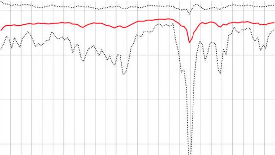
Using this technique, IMF researchers compute the probability distribution of the one-year-ahead forecast for global growth. The solid red line in the chart is the median of this forecast distribution: we can think of this as the central forecast for global growth. The upper and lower dashed lines are the 5th and 95th percentiles of the distribution, respectively. So, for example, in the fourth quarter of 2016, the median forecast for growth in 2017 was 3.67% – that’s the final point on the red line in Figure 1. The dashed lines tell us that the there is a 5% chance that growth will be above 5.58% and a 5% chance that it will be below 2.86%. The lower dashed line – the one that spikes down in late 2008 – is a measure of GDP at risk.
Figure 1 One-year-ahead density forecast for global growth, 1991-2016
Source: IMF (2017), Figure 3.1.2.
Figure 1 also reveals some fundamental properties of the IMF’s estimates. The level of the top dashed line hardly changes. In fact, over the entire 25-year period studied, the 95th percentile of the GDP growth distribution moves between a high of 5.99% and a low of 4.57%. This is in sharp contrast with the measure of GDP at risk (the lower dashed line), which ranges from +3.59% to ‑14.53%. Importantly, these large downward movements are temporary – for most of the period since 1991, GDP at risk is not far below the median.
The asymmetry of the business cycle
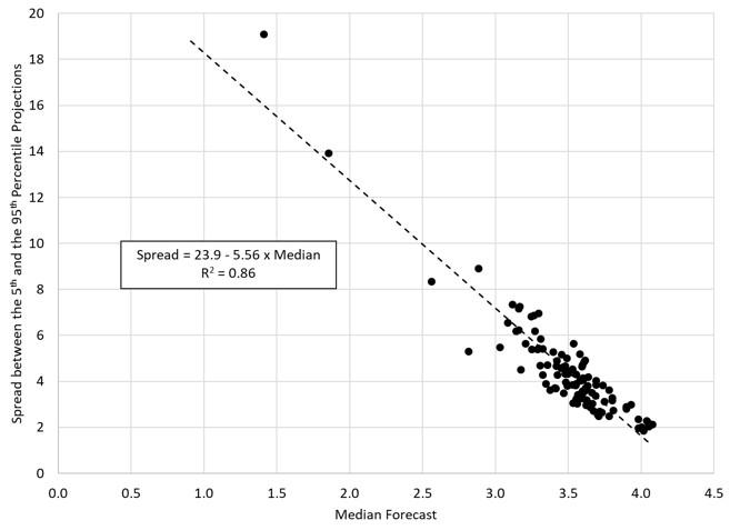
The IMF’s estimates of the growth distribution exhibit an interesting pattern: as the median forecast falls, the forecast distribution widens. This relationship is unlikely to be an accident – increases in uncertainty typically are associated with projections of weaker growth, but (like recessions) these are relatively short in duration. Figure 2 highlights the correlation between the dispersion and the median: a one-percentage point decline in the median forecast (shown on the horizontal axis) is associated with a 5½ percentage point increase in the spread, nearly all of which reflects an increase in GDP at risk. (The fit of the line does not depend on the outliers at the top left.)
Figure 2 One-year-ahead median growth forecasts versus spread
Source: Based on Figure 3.1.2, IMF (2017).
These patterns are consistent with Milton Friedman’s (1993) plucking model of business fluctuations, based on his observation that growth tends to exhibit extended episodes of smooth, upward movement, punctuated by occasional cyclical contractions of shorter duration. That is, business cycles are inherently asymmetric – while the unemployment rate displays temporary jumps in recessions (say, from 5% to 10%), it does not plunge in booms from 5% to 0%. And, usually, it is not very far from 5%.
Why is the lower tail of the growth distribution so much bigger than the upper tail? One explanation starts with the fact that there are short-run constraints such that producing above capacity entails sharply higher costs. By contrast, on the downside, the only limit is that firms shut down. That’s a decline of 100%. Twenty years ago, Kim and Nelson (1999) showed that US GDP exhibits exactly this asymmetry. More recently, Dupraz et al.(2017) develop a model that generates these features.
Toward a financial stability policy framework
We see GDP at risk as a big step forward for policymakers. It is a complement to SRISK, the NYU Stern School Volatility Lab measure of the aggregate capital shortfall in the financial system. In addition to serving as an indicator of financial vulnerability, SRISK also tells us which individual intermediaries are contributing to that vulnerability. GDP at risk helps us to understand the linkages between the financial sector and the real economy at an aggregate level, and can tell us whether an increase in leverage outside of the financial sector increases the likelihood of a severe economic collapse.
GDP at risk has four useful characteristics. First, it is directly based on our ultimate objectives: high real economic growth and low unemployment. These are the foundation for improvements in social welfare.
Second, because GDP already is one of the most widely understood economic concepts, using GDP at risk simplifies policy communication. Imagine two conversations, both between a policymaker and elected officials charged with overseeing the central bank to which they have delegated the role of maintaining financial and economic stability. The first discussion focuses on a measure based on the details of stress tests and network effects – the nuts and bolts of macroprudential policy. The second is anchored by the idea that policymakers should limit the likelihood of an outsized fall in GDP over the next several years. For example, those responsible for policy might say that the odds of a 5% drop over the coming two years should be less than one in ten (i.e. a 10% probability). While technical experts need to have the first conversation among themselves, the second is likely to be much more effective in helping others anticipate policy choices, and in accounting for them after the fact.
Third, provided we accept the centrality of GDP at risk, we can translate much of the machinery of inflation targeting into a financial stability policy framework. Financial Stability Reviews would look like today’s central bank Inflation Reports, with forecasts of GDP at risk at various horizons replacing the path of inflation projections. Of course, such forecasts require an understanding of what makes GDP at risk rise or fall. How important is corporate leverage relative to household leverage? How important are equity versus property price booms? What is the impact of fiscal policy? What types of cross-border capital flows create the biggest vulnerabilities?
Finally, GDP at risk can help discipline discussions of policy trade-offs. At short horizons, central bankers aim to encourage risk-taking when they lower interest rates – faced with an economic slowdown, they wish to stimulate lending. Over longer horizons, however, increased private leverage can create fragilities. So, policymakers want to know the extent to which lower interest rates reduce GDP at risk in the near term, and raise it in the longer term. There are surely many other examples as well.
For several decades prior to the crisis, many central banks with a price stability objective had achieved low and stable inflation. Today, with financial stability taking on such importance, we also expect central bank policies that will lower the probability and the severity of a crisis. But delivering on this means having appropriate risk measures, the tools for maintaining stability, and models that link the two.
GDP at risk is an important step forward in meeting this challenge.
Authors’ note: An earlier version of this column appeared on www.moneyandbanking.com.
References
Adrian, T, N Boyarchenko and D Giannone (2017), “Vulnerable Growth,” Federal Reserve Bank of New York Staff Report No 794, revised November 2017.
Cecchetti, S G (2008), "Measuring the Macroeconomic Risks Posed by Asset Price Booms," in J Y Campbell (ed.), Asset Prices and Monetary Policy, Chicago, IL.: University of Chicago Press, p. 9-43.
Cecchetti, S G and H Li (2008), “Measuring the Impact of Asset Price Booms Using Quantile Vector Autoregressions,” unpublished manuscript, Brandeis International Business School.
Dupraz, S, E Nakamura and J Steinsson (2017), “A Plucking Model of Business Cycles,” unpublished manuscript, Columbia University.
Friedman, M (1993), “The ‘Plucking Model’ of Business Fluctuations Revisited,” Economic Inquiry 31(2): 171-177.
Greenspan, A (2003), “Monetary Policy under Uncertainty,” remarks at a symposium sponsored by the Federal Reserve Bank of Kansas City, Jackson Hole29 August 29.
IMF (2017), Financial Conditions and Growth at Risk, Global Financial Stability Report, October, Chapter 3.
Jorion, P (2000), Value at Risk: The New Benchmark for Managing Financial Risk, 2nd. New York: McGraw-Hill.
Kim, C-J and C R Nelson (1999), “Friedman's Plucking Model of Business Fluctuations: Tests and Estimates of Permanent and Transitory Components,” Journal of Money, Credit and Banking 31(3): 317-334.
Kroenker, R and K F Hallock (2001), “Quantile Regression,” Journal of Economic Perspectives 15(4): 143-156.
Endnotes
[1] The classic reference is Jorion (2000).
[2] See Cecchetti (2006).
[3] For a technical introduction, see Kroenker and Hallock (2001). For an early application, see Cecchetti and Li (2008).


