When markets freeze: Tobin’s q and QE

The economies of the North Atlantic look in poor shape. But it could be worse. Central banks have been doing their best to save capitalism from its own self-fulfilling fears, using the policy of quantitative easing to take frozen assets onto their balance sheets until confidence returns. Why they are doing this – and why it matters – can best be seen in the light of history.

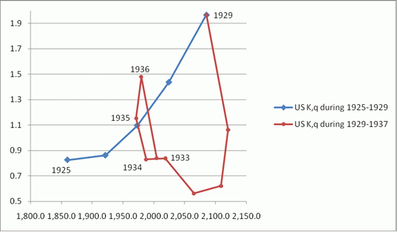
In Lords of Finance: The bankers who broke the world, Liaquat Ahamed provides a graphic account of the inadequate and uncoordinated response by central bankers on both sides of the Atlantic to the US stock market collapse of 1929. Prior to the bust, the US had enjoyed a substantial investment boom – with the real capital stock increasing by more than 3% a year since 1925. But the value of stock market, as measured by Tobin’s q,1 had increased much faster, more than doubling over the same period (see Figure 1).

Figure 1. Capital and real equity prices before and after the 1929 stock market crash

Sources: US Bureau Economic Analysis and Wright (2004)

Then, in two short years, the stock market fell by more than 70%, and the capital stock began to contract – falling by 10% by 1935. These were the years of the Great Depression, when the US banking system collapsed and unemployment grew to over 20% – leading Roosevelt to declare war on unemployment and Keynes to develop his theory of demand-determined output.

Faced with the risk of financial meltdown following the collapse of Lehman Brothers in September 2008, the Federal Reserve, the ECB, and the Bank of England were determined to avoid a repeat of the 1930s – by bailing out the banking system, cutting interest rates to the floor, and buying up frozen assets in what has become known as quantitative easing (QE).

How does QE work? The idea is simple enough: providing cash in exchange for illiquid assets2 should check contraction of investment demand in an economy where there are entrepreneurs who want to invest but lack liquidity – because banks are paralysed by fear of counterparty risk after the collapse of an asset bubble, for example.

In a paper written at the Federal Reserve Bank of NY using a large, calibrated macroeconomic model incorporating the ideas of Kiyotaki and Moore (2008), the results suggest that prompt action by the US Fed – involving the $1 trillion purchase of illiquid assets from the private sector after the collapse of Lehman’s – may have virtually halved the real effects of the liquidity shock in the US. So output fell by 6% rather than 10% (Del Negro et al 2010).

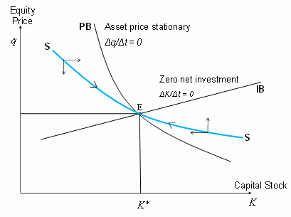
Is there any way for those who do not command the research resources of a Federal Reserve Bank to see how this policy is supposed to work - and when? The answer, we believe, lies in updating the conventional tool of macroeconomics, the Hicksian IS/LM curves dating from 1936! The result of so doing is shown in Figure 2, with Tobin’s q and the capital stock on the axes.

Figure 2. Investment balance, portfolio balance and convergence

While it incorporates intertemporal optimisation by entrepreneurs, the presence of financial frictions – limited resaleability of existing equity and equity-financing limits for new investment – means that Kiyotaki and Moore’s ‘post-Woodford’ approach generates a series of temporary equilibria determined by conditions in money and goods markets. In recent research (Driffill and Miller 2011), we focus on the case of deficient demand. This is indicated in the Figure, where the schedules PB (for portfolio balance) and IB (denoting that investment balances depreciation) are the lines of stationarity for q and K respectively, and the unique path leading to equilibrium at E is shown as SS – with dynamics of adjustment off – equilibrium indicated by the arrows. While this may be reminiscent of Hicks’s IS/LM interpretation of Keynes, there are obvious points of difference:

• It is an asset price not an interest rate on the vertical axis

• The stock of capital not the level of national income is on the horizontal axis; and

• There are explicit dynamics of adjustment.

But the level of income depends on current investment in a rather Keynesian fashion, nonetheless.

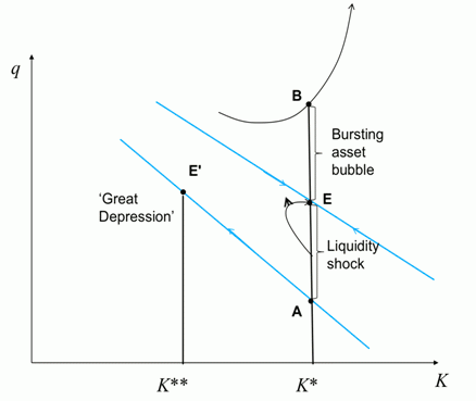
What then is the impact of tightening credit constraints – a liquidity shock? This is the question the FRB New York faced, and the answer is indicated in Figure 3. Because it makes equities less attractive and investment more difficult, it will move the lines of stationarity so that equilibrium shifts from E to E’ – to be approached in turn by a process of adjustment starting at point A as indicated. There will be an immediate fall of asset prices and investment, and, because national income depends on investment, an immediate economic contraction.

Figure 3. Bursting of asset bubble and liquidity contraction: a case for QE?

In fact, liquidity shocks often come in the aftermath of collapsing asset prices, as in the 1930s. This feature is also indicated in Figure 3 by the ‘off-equilibrium’ path of rising asset prices and booming investment characterising the economy before the bubble bursts (when assets are overvalued by BE).

Taking no action when the bubble bursts – with the knock-on effect of a liquidity shock that takes asset values down to A – could lead to a sustained fall in investment and output. So the capital stock could contract substantially, to E’, the point labelled as “Great Depression”. If illiquidity of capital were the only problem, then an immediate open market purchase of illiquid equity assets by the central bank, to be held until such time as confidence returns, could in principle avert the contraction and keep the economy at E. Troubles seldom come in single file, however, so much more may need to be done – recapitalising banks for instance.

 A partial reversal of the initial liquidity shock by the purchase of a fraction of the illiquid capital can limit the damage, however, as indicated by the path labelled QE in the figure reflecting expected mean reversion in credit conditions. This appears to be what the US central bank did to engineer what the FRB New York team call the “Great Escape”. It is surely no coincidence that the Chairman of the Fed won his academic spurs with research on the importance of credit conditions in accounting for the Great Depression.

In historical perspective, it was President Roosevelt’s willingness to challenge the established precepts of a balanced budget and a fixed price of gold that helped the US recover from the Great Depression. Is the willingness of central bankers to step outside the usual rules of the game to so as preempt economic collapse the modern equivalent of FDR’s activism? For, in recent times, central banks have far exceeded their customary remit, acting not only as lenders of last resort but also as market makers and, in conjunction with the treasury, as suppliers of capital too.

The key element causing the crisis of illiquidity in 2008-09 was uncertainty over the value of US subprime mortgages; and asset-backed and mortgage-backed securities were a major element of Fed purchases. In the current Eurozone crisis, however, it is the sovereign debt of southern member states (and the liabilities of banks with large exposure) that is the immediate threat to liquidity. According to some observers, the challenge facing the ECB is whether – and on what terms – it should take up these illiquid assets in what would amount to another spectacular act of quantitative easing.

Ahamed, Liaquat (2009), Lords of Finance: The bankers who broke the world. London: William Heinemann

Driffill, John and Marcus Miller (2011), “Liquidity when it matters most: QE and Tobin’s q”, CEPR DP No. 8511.

Del Negro, Marco, Gauti Eggertsson, Andrea Ferrero and Nobuhiro Kiyotaki (2010), “The Great Escape? A Quantitative Evaluation of the Fed's Non-Standard Policies”, FRB NY working paper.

Kiyotaki, Nobuhiro, and John Moore (2008), “Liquidity, Business Cycles, and Monetary Policy”. Mimeo: Princeton, Edinburgh and LSE.