Imagine you want to reduce greenhouse gas emissions to stabilise climate change. Reviewing your options, you find that efficiency opportunities in the building sector can reduce emissions for $12 per avoided tonne of carbon. Other options, such as transforming transport with electric vehicles or public transit, would reduce emissions for almost twice the price – say, $21 per tonne of avoided carbon. Which option should you chose?
The question may seem silly, and the answer obvious. Traditional climate economics models recommend capturing the cheapest opportunities to reduce emissions first – the ‘low hanging fruits’ – and keeping the most difficult options for later. This approach sounds like common sense, and it is at the basis of the ‘marginal abatement cost curves’ (MACCs) approach (McKinsey and Company 2009).
But common sense sometimes gets it wrong. As is well known, investing early in relatively expensive emission-reduction options can be justified based on a technological rationale. Specifically, through learning, investing in expensive technologies would lower their cost over the long term (Wigley et al. 1996, Goulder and Mathai 2000, Bramoullé and Olson 2005, Kverndokk and Rosendahl 2007, del Rio Gonzalez 2008, Acemoglu et al. 2012, Creti et al. 2017). Indeed, it may well make sense to invest in offshore windmills even if they are more expensive than onshore windmills or solar panels, in the hope that these investments will reduce the cost of offshore wind, making it a competitive renewable energy option in the future.
Our recent paper (Vogt-Schilb et al. 2018) provides another – independent – rationale for investing early in relatively expensive emission-reduction options. Our study represents emissions reductions more realistically than in previous works, by modelling the fact that reducing emissions takes time and requires investments in long-lived goods and assets. It concludes that, even when no technical change is expected, it makes sense to start reducing emissions in the sectors where doing so is the most expensive and the most difficult, leaving the easier things for later.
Why such a counter-intuitive result? It’s actually simple. In most sectors, an abrupt transformation would be more expensive than a smooth shift towards zero net emissions. In sectors that are particularly expensive and difficult to decarbonise, like transportation, it is therefore preferable to start early to make the transformation as progressive and smooth as possible, minimising long-term costs. Even if technologies used in urban transportation are not expected to improve over time, policymakers may want to start early, given that transforming transportation systems gradually is cheaper than doing so quickly later on.
The recommendations of the traditional model are unrealistic
The canonical climate economics model in academia originates from Nordhaus (1991), and has been used for nearly three decades to provide insights into efficient emission-reduction policies (Dietz and Stern 2014). It relies on MACCs, which provide information on abatement potential and costs for a set of technical mitigation measures for a given date (McKinsey and Company 2009). It assumes that agents can decide by how much to reduce emissions, independently, every day. And the more agents want to reduce emissions, the more expensive it becomes to reduce emissions by one more tonne – in economic terms, the marginal cost of reducing emissions is increasing.
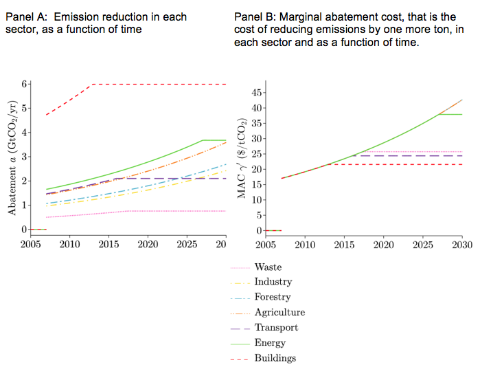
As an illustration, Figure 1 shows the optimal timing and cost of emission reductions according to this classical model, assuming that the objective is to keep the emissions over the 2007-2030 period at a level consistent with the 2º centigrade target of the Paris Agreement. The marginal abatement cost curves are calibrated with Intergovernmental Panel on Climate Change (IPCC) data. These numbers are strictly illustrative, since this simulation ends in 2030, while an optimal strategy would need to consider a longer time scale, and because abatement costs have decreased a lot since these data were collected. Even so, they are sufficient to make our case.
In panel A, we see that this model recommends reducing emissions immediately in the cheapest sector (here, a reduction by almost 5 billion tons of CO2 the first year in the building sector), and to start more slowly in the more expensive sectors (like transport and industries). Once all options to reduce emissions have been used in a given sector (for instance, once all buildings are retrofitted), efforts in that sector plateau, and increase in other, more expensive sectors. At each point in time, more emission reductions are done in the sectors where it is the cheapest, reflecting the fact that all sectors reduce emissions at the same marginal cost, as seen in Panel B.
Figure 1 Optimal timing and cost of emission reductions in the traditional model
Note: MAC is the marginal adjustment cost for each sector – it is the same for all sectors.
But we argue that the recommendations of the traditional model are unrealistic. It recommends a drastic reduction in emissions in the building sector, by magically retrofitting 80% of buildings overnight. This happens because MACCs do not convey information on the time dimension – that is, how long it takes to implement a measure, and how the cost depends on the time it takes to implement a measure. Another oddity is that in the traditional model, if we were to stop paying for emission reductions after a couple of decades, then emissions would return to their baseline level immediately. For example, if climate change policies were repealed 20 years from now, emissions would instantaneously return to the level they would have been in 2038 in the absence of those policies. This absurd outcome is the result of an absence of the time dimension (‘inertia’) in the model of the system – emission reductions are determined each year independently.
Our model represents emission reduction decisions as investments with long-term consequences
Given the shortcomings of the traditional model, our model introduces a very simple tweak to make it more realistic, by representing emission reductions as investments. Now agents cannot directly decide every year how much to reduce emissions. But they can decide every year how much emission reduction equipment to build – for example, items such as electric cars, building insulation, windmills, or metro lines, that will stick around for decades to centuries once built.
We also introduce nonlinear investment costs, often called ‘adjustment costs’ by economists (Lucas 1967). Low-carbon investments are more expensive if they are rushed than if they are smoothed over time. Imagine you want to retrofit all buildings in a country with great thermal insulation and efficient appliances. It would be cheaper to do that over a couple of decades, making use of the existing industry and skilled workers, rather than rushing it over a single year, which could require diverting a substantial share of the workforce and capital away from other productive uses in the economy.
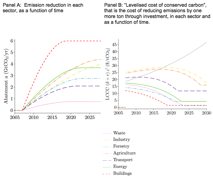
Figure 2 shows the optimal timing and cost of emission reductions with the same objective as in Figure 1, but according to our new model. In panel A, we see that emissions do not ‘jump’ anymore, and it takes years of investment to achieve significant emission reductions.
Figure 2 Optimal emission reduction strategy with investments in emission reduction in our model
Note: LCCC is the ‘levelised’ cost of conserved carbon (the cost paid for the last ton of emission that is avoided) and is the equivalent to the marginal abatement cost in our model. It varies by sector and follows a bell-shape trajectory.
We see also that the cost of reducing emissions is different across sectors, and it follows a bell-shape curve instead of increasing regularly over time. This optimal strategy, using the same IPCC calibration as before, looks more realistic, with smoother, progressive decarbonisation strategies. Now years of climate policies also have a long-term impact. For example, if we stopped investing in emission reductions after 20 years, emissions would remain for years at a level that is lower than what they would have been if no policy had been implemented in the first place – thanks to all the low-carbon equipment that would be present after 20 years of climate policies.
Most importantly, the optimal emission-reduction strategy is now completely different. First, the strategy looks much more like a transition, with large investments at the beginning to transform the economic system, and smaller efforts over the long term.
Second, the strategy calls for a very different allocation of efforts across sectors, with immediate and large investments in sectors with long-term potential (such as transportation or industry). In particular, the optimal solution is to invest in options with a higher cost, in the sectors where reducing investment is more expensive. For instance, an investment that cost $21 per tonne in the transport sector makes sense, even if alternative options exist at $12 in the building sector. The rationale is that since the transport sector is difficult and expensive to decarbonise, policymakers should spread the effort over time, even if it means accepting higher costs per ton of emission reductions in the short term.
It does not make sense to compare options to reduce emissions solely on their cost
While our numerical results are only illustrative, they have important policy and operational implications. They show that it makes no sense to compare options to reduce emissions solely on marginal abatement costs. A policy that reduces emissions at a cost of $100 per avoided tonne may be desirable – even if other options exist to reduce emissions at $20 per tonne – if investing now at $100 per tonne prevents the need to reduce emissions later in a rush at a much higher cost. As already stated, investing early in relatively expensive emission reduction options can also be justified by the benefits from induced technical change. In the real world, the two arguments add up – early investments make sense in sectors that are long and expensive to decarbonise, and in sectors where we expect a lot of technological progress to happen as countries invest.
In sum, our recommendations are different than those that stem from the traditional abatement cost curve model. We argue that instead of selecting the lowest cost options every day, there is a need to work backwards from the long-term objective of reaching zero net emissions, and think today about the short-term decarbonisation pathways that can put the economy on track to reach this goal at the lowest possible cost, as follows (Clarke et al. 2014, Fay et al. 2015, Bataille et al. 2016).
- First, policymakers need to consider a long-term objective consistent with the Paris Agreement, such as reducing emissions by 50% by 2050.
- Next, they can identify what needs to happen to achieve these objectives in every sector and derive sectoral objectives. For instance, reducing emissions by 50% may require retrofitting all buildings and transforming transportation systems.
- Then, they should analyse what actionable short-term targets would put their country on track to achieve these sectoral objectives at the lowest possible cost. For instance, retrofitting all buildings by 2050 may be achieved at the lowest cost if they start investing a significant amount of resources by 2020.
- The final step would be to design the combination of policies and measures – from performance standards to innovation subsidies and infrastructure investment – that are able to effectively deliver those targets (Altenburg et al. 2017).
Typically, this approach will result in a recommendation not to delay action in the sectors that are the most expensive and difficult to decarbonise, especially as far as long-lived infrastructure systems are involved. For example, it will not be possible to transform cities in just a couple of decades – not at an acceptable cost. Thus, actions on urban planning and urban transport systems are especially urgent.
References
Acemoglu, D, P Aghion, L Bursztyn, and D Hemous (2012), “The Environment and Directed Technical Change”, American Economic Review, 102 (1), 131–66.
Altenburg, T, C Assmann, D Rodrik, E Padilla, S Ambec, M Esposito, A Haider, W Semmler, D Samaan, and A Cosbey (2017), “Green Industrial Policy: Concept, Policies, Country Experiences”.
Bataille, C, H Waisman, M Colombier, L Segafredo, J Williams, and F Jotzo (2016), “The Need for National Deep Decarbonization Pathways for Effective Climate Policy”, Climate Policy, 16 (sup1), S7–26.
Bramoullé, Y, and L J Olson (2005), “Allocation of Pollution Abatement under Learning by Doing”, Journal of Public Economics, 89 (9–10), 1935–60.
Clarke, L, K Jiang, K Akimoto, M Babiker, G Blanford, K Fisher-Vanden, J C Hourcade, V Krey, E Kriegler, and A Loeschel (2014), “Assessing Transformation Pathways”, In O Edenhofer, R Pichs-Madruga, Y Sokona, E Farahani, S Kadner, K Seyboth, A Adler, I Baum, S Brunner, P Eickemeier, B Kriemann, J Savolainen, S Schlömer, C von Stechow, T Zwickel and J C Minx (eds.), Climate Change 2014: Mitigation of Climate Change, Working Group III Contribution to the IPCC 5th Assessment Report, Cambridge, United Kingdom and New York, NY, USA: Cambridge University Press.
Creti, A, A Kotelnikova, G Meunier, and J-P Ponssard (2017), “Defining the Abatement Cost in Presence of Learning-by-Doing: Application to the Fuel Cell Electric Vehicle”, Environmental and Resource Economics, September, 1–24.
Dietz, S, and N Stern (2014), “Endogenous Growth, Convexity of Damages and Climate Risk: How Nordhaus’ Framework Supports Deep Cuts in Carbon Emissions”, Economic Journal, June.
Fay, M, S Hallegatte, A Vogt-Schilb, J Rozenberg, U Narloch, and T Kerr (2015), Decarbonizing Development: Three Steps to a Zero-Carbon Future, Washington DC, USA: World Bank Publications.
Goulder, L H, and K Mathai (2000), “Optimal CO₂ Abatement in the Presence of Induced Technological Change”, Journal of Environmental Economics and Management, 39 (1), 1–38.
Kverndokk, S, and K E Rosendahl (2007), “Climate Policies and Learning by Doing: Impacts and Timing of Technology Subsidies”, Resource and Energy Economics, 29 (1), 58–82.
Lucas, R E, Jr (1967), “Adjustment Costs and the Theory of Supply”, Journal of Political Economy, 75 (4), 321–34.
McKinsey and Company (2009), “Pathways to a Low-Carbon Economy: Version 2 Og the Global Greenhouse Gas Abatement Cost Curve”.
Nordhaus, W D (1991), “A Sketch of the Economics of the Greenhouse Effect”, The American Economic Review, 81 (2), 146–150.
Rio Gonzalez, P del (2008), “Policy Implications of Potential Conflicts between Short-Term and Long-Term Efficiency in CO2 Emissions Abatement”, Ecological Economics, 65 (2), 292–303.
Vogt-Schilb, A, G Meunier, and S Hallegatte (2018), “When Starting with the Most Expensive Option Makes Sense: Optimal Timing, Cost and Sectoral Allocation of Abatement Investment”, Journal of Environmental Economics and Management, 88 (March), 210–33.
Wigley, T M L, R Richels, and J A Edmonds (1996), “Economic and Environmental Choices in the Stabilization of Atmospheric CO2 Concentrations”, Nature, 379 (6562), 240–243.


