Housing supply elasticities – the response by builders to a change in house prices – help explain why house prices differ across locations (Green et al. 2005). The more inelastic housing supply becomes, the more rising demand translates into rising prices and the less into additional housebuilding. In a new paper, we use a rich US dataset and novel identification method to show that supply elasticities vary across cities and across time (Aastveit et al. 2020). We find that US housing supply has become less elastic since the crisis, with bigger declines in places where land-use regulation has tightened the most and in areas that had larger price declines during the crisis. This new lower elasticity means US house prices should be more sensitive to changes in demand than before the crisis.
The 1996-2006 boom versus the 2012-2017 recovery
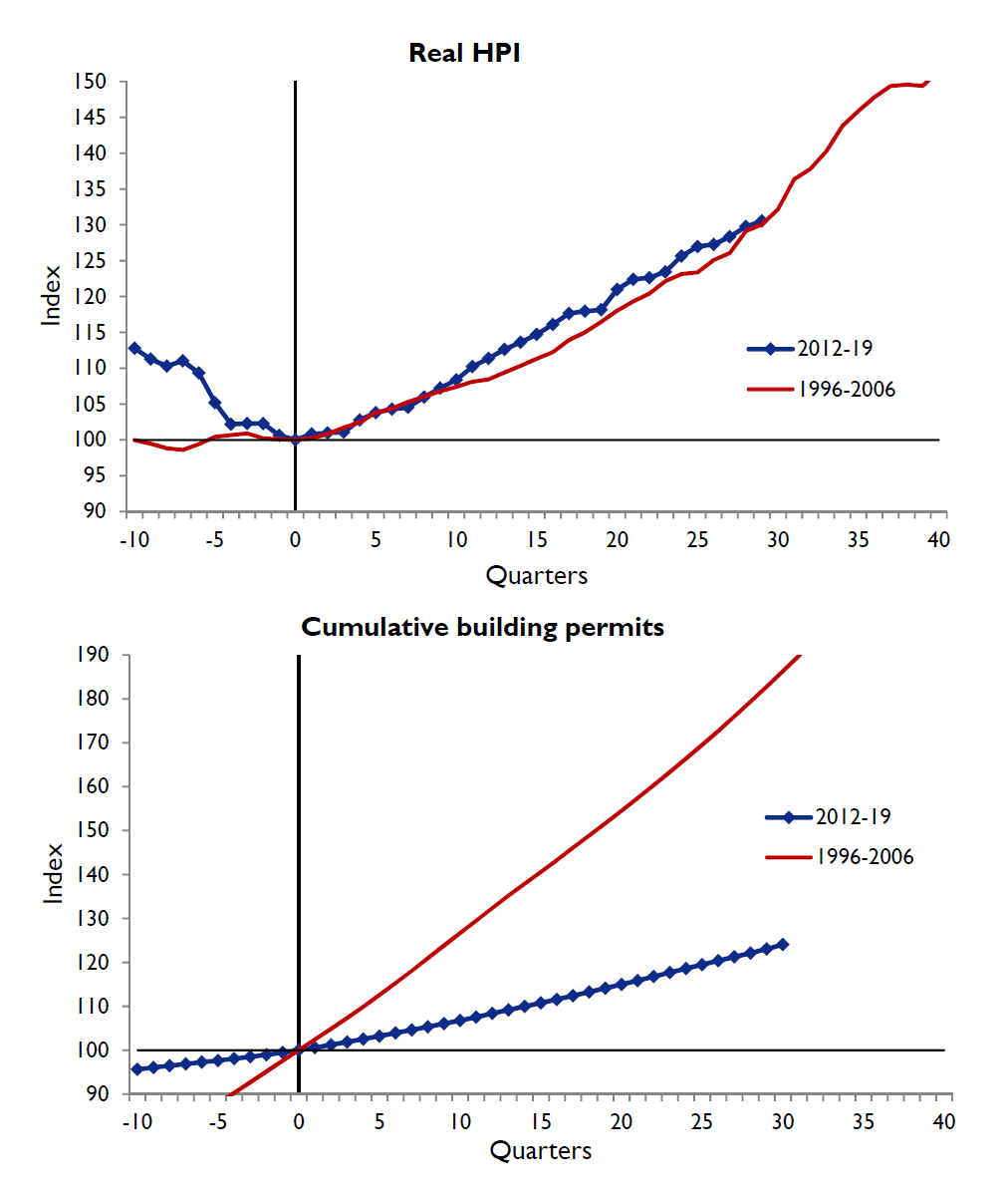
House prices in the US have increased by roughly 30% in real terms since the housing recovery started in mid-2012, a remarkably similar pattern to the 1996-2006 housing boom (top panel of Figure 1). But despite similar developments in house prices, housing supply has grown substantially less during the current housing expansion. While the cumulative increase in building permits between 2012 and 2019 has been just above 20%, the comparable figure for the previous boom is roughly 86% (bottom panel of Figure 1). Our measure of housing supply is building permits – an authorisation granted by local governments or other regulatory bodies before construction of a new or existing building start – but housing starts and housing completions display similar trends.
Figure 1 House price developments across booms
Sources: Bureau of Labor Statistics, Census Bureau, Federal Housing Finance Agency, and authors’ calculations.
Notes: The figure shows developments in the FHFA house price index deflated by the Consumer Price Index, and building permits during 1996q4–2006q4 (red solid line) and 2012q3–2019q3 (blue line with markers). The series are scaled such that they take a value of 100 at the beginning of both periods. The horizontal axis shows quarters around the beginning of the two booms, and the vertical line at zero is the starting point of both booms.
We have two housing booms (or expansions) with similar price developments but a much weaker recovery in construction this time around. This suggests that the US housing supply elasticity – i.e. the response of housing supply to a given change in house prices – has declined. In other words, our hypothesis is that home builders may have become less price-responsive compared to the housing market expansion in the run-up to the Great Recession.
In this column, we tackle the following three questions:
- How have housing supply elasticities evolved across the US since the Great Recession?
- What accounts for the change in supply elasticities?
- What are the potential implications for the transmission of housing demand shocks?
Main framework to estimate local housing supply elasticities
The housing market is seen as a collection of several markets that differ not only in terms of geography but also in other attributes, resulting in significant differential regional house price performance (Ferreira and Gyourko 2012, Piazzesi and Schneider 2016). One of the dimensions that better explains these differences in house prices is geographical (Saiz 2010) and regulatory supply restrictions (Gyourko et al. 2008). We stress in our paper that the marked differences in housing market developments across US Metropolitan Statistical Areas (MSAs)1 should be taken into account to provide a better picture about the state of the US housing market.
Our quarterly panel data set covers 254 US MSAs, spanning the previous boom (1996-2006) and the recent recovery (2012-2017). We stop in 2017 due to data availability issues for some key variables. We estimate local housing supply elasticities for each of the sub-samples through a single-equation approach (Green et al. 2005). The idea is to estimate how supply (i.e. building permits) responds to house prices, after controlling for several local economic and socio-demographic variables. We also allow supply elasticities to vary conditional on supply restrictions. We measure topographical restrictions with Saiz’s (2010) UNAVAL Index, which uses GIS and satellite information to calculate the share of land in a 50 km radius of the main city centre that is covered by water, or where the land has a slope exceeding 15 degrees. We measure regulatory constraints using the Wharton Regulatory Land Use Index (WRLURI) from Gyourko et al. (2008), which measures the stringency of local zoning laws (i.e. the time and financial cost of acquiring building permits and constructing a new home). Overall, we expect areas with tighter geographical and regulatory restrictions to expand supply less for the same change in house prices.
Instrumental variable identification
Before estimating the housing supply equation for each housing boom period, we need to address the issue of reverse causality, whereby the direction of causality can also run from building permits to house prices. Standard textbook economics would tell us that higher supply (construction) in the market may dampen (house) prices. Our aim is to estimate how supply reacts to a demand-driven change in house prices, not by supply itself. Our identification problem thus requires separating housing demand from housing supply.
We use an instrumental variable (IV) approach, with two instruments for house prices that we argue lead to shifts in housing demand but that do not shift housing supply. The first one is crime rates compiled by the FBI. Given the significant negative impact that crime can have on society, it can be viewed as an exogenous negative amenity that drives house price changes both within and across MSAs (Pope and Pope 2012). The second instrument is real personal disposable income. Income is one of the main determinants of housing and consumption demand in standard macro and housing models, and typically does not affect housing supply directly (Meen 1990, Muellbauer and Murphy 1997, Meen 2001, Duca et al. 2011).
Estimated elasticities
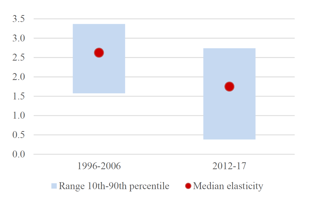
Our IV estimates suggest that supply elasticities have fallen across the board since the last housing boom (Figure 2). For instance, the median MSA in the sample experienced a decline in elasticity from 2.63 during the 1996-2006 housing boom to 1.75 during 2012-17. In other words, a 1% rise in local house prices would lead to a 1.75% increase in permits now for the median elasticity area, compared to 2.63% in the previous boom. Moreover, the dispersion in supply elasticities appears to have increased during the current cycle, as evidenced by a particularly strong decline in the elasticities for the lowest part of the distribution.
Figure 2 Estimated housing supply elasticities
Notes: The red dots refer to the median estimated elasticities for each housing boom, while the blue bars show the 10th-90th percentile range.
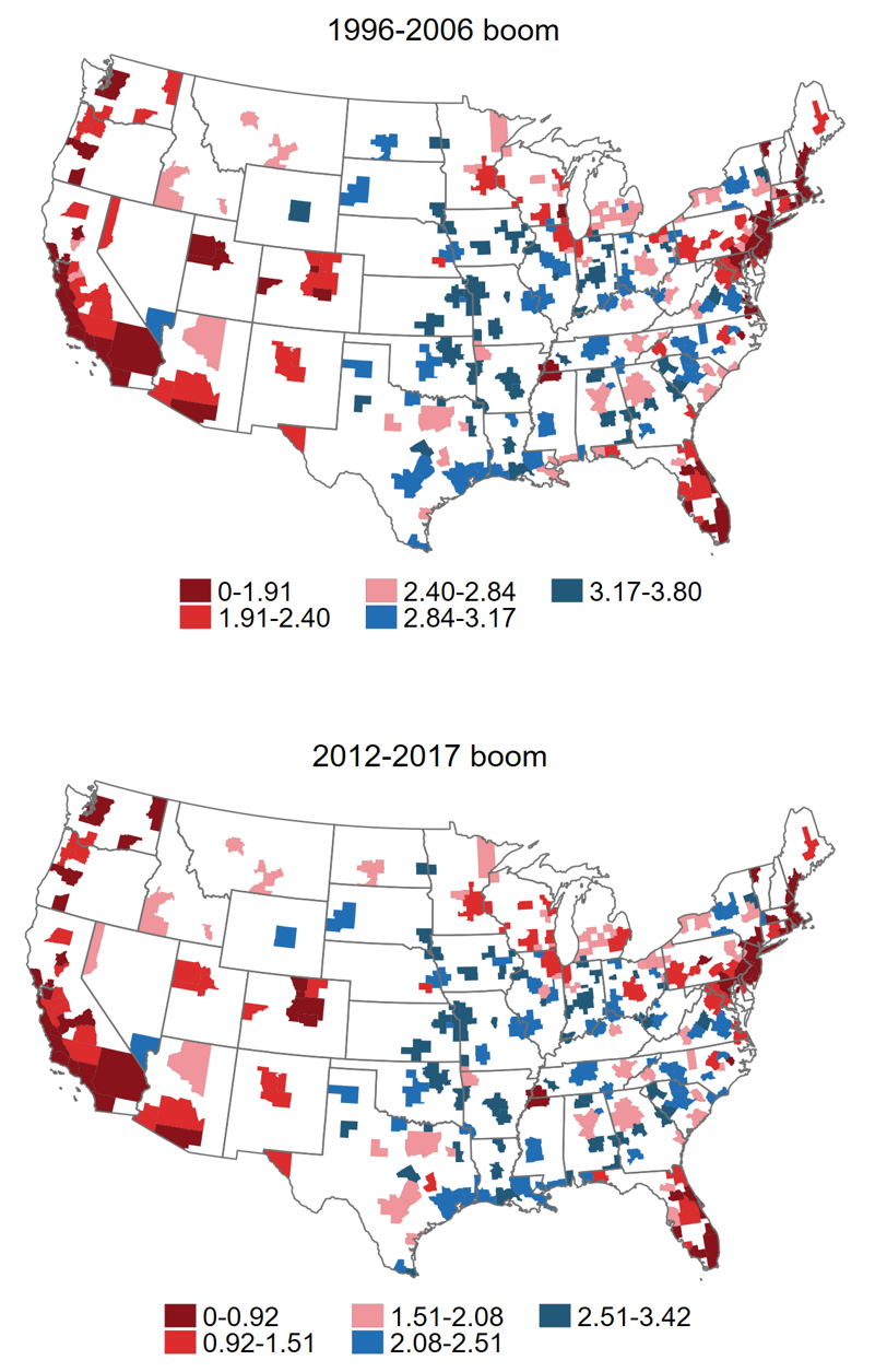
Housing supply elasticities are characterised by considerable heterogeneity across MSAs (Figure 3). For example, areas located in states such as California, Arizona, Florida, and New York exhibit the lowest elasticities in both booms. This is not surprising, given that geographical idiosyncrasies, such as steep ground and bodies of water, make it harder to build and limit the land available for construction (Saiz 2010). In addition, land-use regulation also tends to be more stringent in these areas (Gyourko et al. 2008). By contrast, we estimate high-elasticity areas to be located in the Midwest, where builders tend to face relatively fewer restrictions to expanding housing supply.
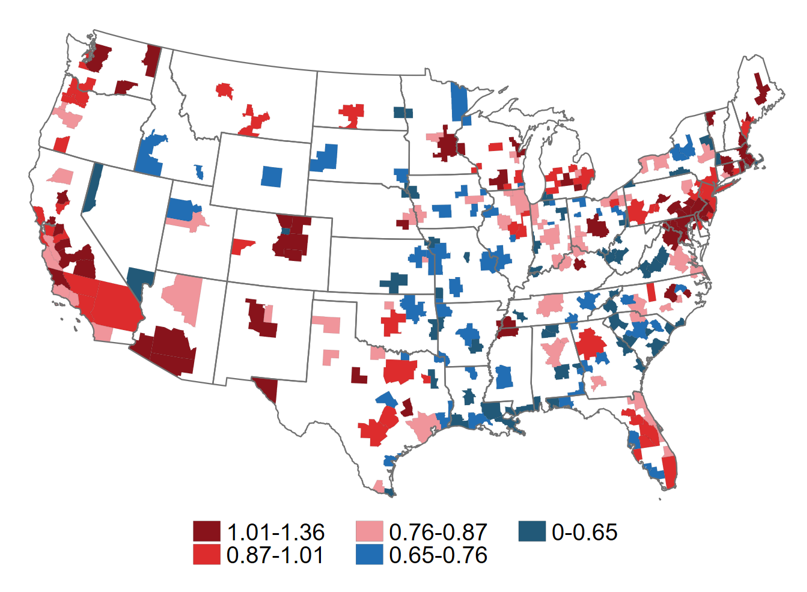
In addition to the cross-sectional variation, we also find that there are regional differences in the extent of the decline in supply elasticities. Specifically, areas that had the lowest elasticities during the first housing boom, predominantly coastal areas, experienced the largest decline in elasticities between the two booms (Figure 4).
Figure 3 Estimated elasticities for the two housing booms
Notes: Estimated elasticities for each housing boom. Smaller values refer to lower elasticity areas.
Figure 4 Decline in estimated elasticities between booms
Notes: The figure shows the decline in the estimated elasticities between the two housing booms.
Why have elasticities declined?
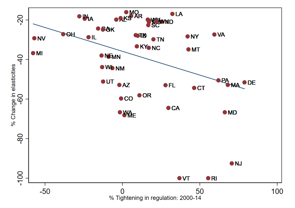
Although it is challenging to pin down the reasons behind the generalised decline in supply elasticities, we argue that tighter land-use regulation and precautionary motives may have played a role. More precisely, Figure 5 shows that we find that elasticities have declined the most in areas where regulation has tightened more (Herkenhoff et al. 2018) and in areas that experienced the largest declines in house prices during the Great Recession. We interpret the latter as evidence that the fear of a new bust has led developers to be less price-responsive than before.
Figure 5 Correlation between changes in estimated supply elasticities and changes in land-use regulation in each state
We believe there may be other alternative explanations for the weaker response of supply to house prices, such as increased market concentration in the home building sector after the Great Recession (Haughwout et al. 2012), increasingly scarcer land (JCHS 2018), and stricter capital requirements on loans extended to construction and land development.
The consequences of lower supply elasticities
Keeping track of changes in the housing market structure is key to understanding how demand shocks transmit to the real economy over time. The theoretical assumption is that lower supply elasticities imply that a given change in demand should have a stronger effect on house prices and a weaker effect on quantity.
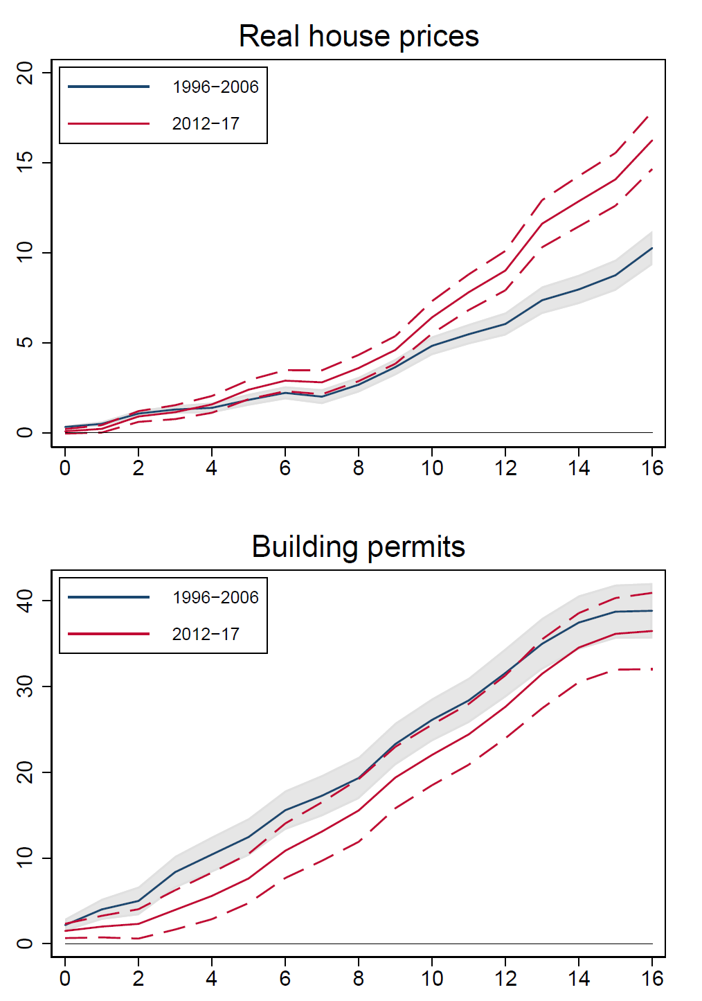
We explore the relevance of this conjecture using state-of-the-art exogenous monetary policy shocks as a proxy for shifts in housing demand (Gertler and Karadi 2015). We then explore how these shocks affect house prices and supply across the two booms. Our estimates suggest that, following an expansionary 100 basis point monetary policy shock, house prices rise by considerably more during 2012-2017 compared with the 1996-2006 boom (upper panel of Figure 6): real house prices in the current boom are 6 percentage points higher after four years. We estimate the opposite dynamics for building permits.
Figure 6 Impulse responses to an expansionary monetary policy shock across booms
Notes: Cumulative impulse responses to a monetary policy shock calibrated to induce a 100 basis point decline in the one-year Treasury bill yield, assessed at the sample median elasticity for each housing boom period. The x-axis refers to quarters, and the y-axis to % changes. The grey area and the dashed red lines refer to 90 percent confidence bands.
Further thoughts
The decline in US housing supply elasticities may explain why recent research has found that monetary policy may have become more effective for financial variables (Paul 2020) – an aggregate shock that raises housing demand is absorbed mostly by price adjustments, rather than quantity adjustments. This finding may be important for financial stability considerations, whereby policy actions that stimulate (housing) demand may have unintended effects by raising house prices. Although it remains to be seen whether the decline in the elasticities is permanent or transitory, increasingly tighter land-use regulation suggests that it may be more challenging to go back to pre-crisis supply elasticities.
Authors’ note: The views expressed in this column should not be reported as representing the views of Norges Bank or the Bank of England.
References
Aastveit, K A, B Albuquerque and A Anundsen (2020), “Changing supply elasticities and regional housing booms”, Bank of England Staff Working Paper 844.
Duca, J, J Muellbauer and A Murphy (2011), “House prices and credit constraints: Making sense of the US experience”, Economic Journal 121: 533–551.
Ferreira, F and J Gyourko (2012), “Heterogeneity in Neighborhood-Level Price Growth in the United States, 1993-2009”, American Economic Review 102(3): 134–140.
Gertler, M and P Karadi (2015), “Monetary Policy Surprises, Credit Costs, and Economic Activity”, American Economic Journal: Macroeconomics 7(1): 44–76.
Green, R K, S Malpezzi and S K Mayo (2005), “Metropolitan-Specific Estimates of the Price Elasticity of Supply of Housing, and Their Sources”, American Economic Review 95(2): 334–339.
Gyourko, J, A Saiz and A Summers (2008), “A New Measure of the Local Regulatory Environment for Housing Markets: The Wharton Residential Land Use Regulatory Index”, Urban Studies 45(3): 693–729.
Haughwout, A, R W Peach, J Sporn and J Tracy (2012), “The Supply Side of the Housing Boom and Bust of the 2000s”, in Housing and the Financial Crisis, NBER Chapters, pp. 69–104.
Herkenhoff, K F, L E Ohanian and E C Prescott (2018), “Tarnishing the Golden and Empire States: Land-Use Restrictions and the U.S. Economic Slowdown”, Journal of Monetary Economics 93: 89–109.
JCHS (2018), The State of the Nation’s Housing, technical report, Joint Center for Housing Studies of Harvard University.
Meen, G (1990), “The removal of mortgage market constraints and the implications for econometric modelling of UK house prices”, Oxford Bulletin of Economics and Statistics 52(1): 1–23.
Meen, G (2001), Modelling Spatial Housing Markets: Theory, Analysis and Policy, Kluwer Academic Publishers.
Muellbauer, J and A Murphy (1997), “Booms and busts in the UK housing market”, Economic Journal 107(445): 1701–1727.
Saiz, A (2010), “The Geographic Determinants of Housing Supply”, The Quarterly Journal of Economics 125(3): 1253–1296.
Paul, P (2020), “The Time-Varying Effect of Monetary Policy on Asset Prices”, The Review of Economics and Statistics (forthcoming).
Piazzesi, M and M Schneider (2016), Housing and Macroeconomics, Vol. 2 of Handbook of Macroeconomics, Elsevier, pp. 1547–1640.
Pope, D G and J C Pope (2012), “Crime and property values: Evidence from the 1990s crime drop”, Regional Science and Urban Economics 42(1-2): 177–188.
Endnotes
1 Groups of cities with a high degree of economic and social integration, where at least one city has 50,000 or more inhabitants; see https://www.census.gov/programs-surveys/metro-micro/about.html


