Since March 2020, there has been an explosion of research by economists on COVID-19. A typical analysis posits an economy that is subject to epidemiological dynamics, but in many cases, this modelling is erroneous. These errors have important consequences for optimal economic planning and for COVID-19-related policymaking. In particular, the disease is erroneously characterised as relatively slow moving, which distorts policymaking toward less severe, delayed interventions such as delayed lockdowns. Moreover, the scale of the disease is underestimated.
In Bar-On et al. (2020a), we elaborate the correct model that needs to be used and the reasons for the errors made by many economists. We base our discussion on the epidemiological analysis of COVID-19 and, in particular, on transmission timescales.
A model based on the epidemiological evidence
To understand the common errors, consider what a correctly-specified model needs to look like. The following is based on the latest epidemiological and clinical evidence available on SARS-CoV-2 (drawing on Bar-On et al. 2020b). We model two blocks: an infection transmission block and a clinical block.
Infection transmission: The SEIR-Erlang model
In this first block, modelling follows the well-known compartmental model approach proposed by Kermack and McKendrick (1927). The time profile of an individual follows distinct stages, or compartments, moving from Susceptible (S) to Exposed (E) to Infectious (I) and to Resolved (R); hence, the name SEIR.
In both the Exposed and Resolved compartments, infectiousness is zero; infectiousness happens only in the Infectious compartment. An individual spends a certain amount of time in each compartment before moving to the next compartment. The times spent in the Exposed and Infectious compartments are known as the latent1 and infectious periods, respectively.
A simple compartmental model describes exponentially distributed latent and infectious periods. This model reflects three key epidemiological properties of COVID-19: (i) People who get infected are not immediately infectious as there is a latent period at the beginning of the disease (denoted E, standing for ‘exposed’). (ii) On average, people are infectious for a few days only. (iii) After that, one does not transmit the disease anymore even though the disease continues, and it might take quite some time until one recovers or dies.
On average, the latent period lasts for 3-4 days and the infectious period for 4-5 days, with the modes of the Exposed and Infectious duration distributions near their means. Using sub-compartments is necessary to match this feature, and the model with sub-compartments is called SEIR-Erlang (see Bar-On et al. 2020a for details).2
Figure 1a depicts the model. It indicates the number of days it takes to pass from one compartment to the other in days, based on epidemiological studies.
Figure 1a The infection transmission block
Notes: S denotes susceptible, E1 and E2 denote the two sub-compartments of the latent stage, I1 and I2 denote the two sub-compartments of the infectious stage, R denotes resolved.
Dynamics within the public health system: The clinical block
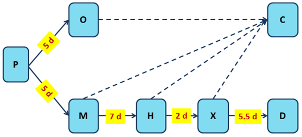
As an infected person progresses through the compartments shown in Figure 1a, they go through the clinical stages handled by the public health system. This process depends on the development of symptoms and their severity. The onset of symptoms and subsequent clinical developments follow a separate timeline from the infection-spreading timeline described above. We therefore suggest to describe it by the following clinical block, with average durations in days:
Figure 1b The clinical block
Notes: P denotes the incubation period, O denotes asymptomatic, M denotes the period between the onset of symptoms and hospitalisation, H denotes hospitalisation stay till admission to ICU, X denotes time in ICU till death (D) or recovery (C).
The durations shown in Figure 1b (in days) are based on clinical studies referenced in Bar-On et al. 2020a.
As is evident from panels a and b of Figure 1, disease transmission and clinical progression follow independent timelines. This distinction determines the way the model is parameterised. We focus on one central element of the parameterisation and refer the reader to Bar-On et al. (2020a) for a detailed discussion.
Comparison to the misspecified model
Economists most commonly use the well-known SIR epidemiological model, which looks like Figure 1a without the Exposed compartment and with a single compartment for Infectious. In calibrating this model, researchers consider two main targets: (i) a value for the basic reproduction number R; and (ii) disease duration till death, usually assumed to be 18-19 days.
The key feature of the model in Figure 1 is that it allows calibrating the parameters related to disease transmission separately from the parameters related to its clinical outcomes (such as the duration of the disease). In particular, the duration of the infectious stage is parameterised to be 4 days in line with epidemiological evidence, whereas the total duration of disease till death is described in the clinical block, based on clinical evidence, and is set at 19.5 days. This is not the case in the widely-used SIR parameterisation, which confounds the total duration of the disease with the infectiousness period and assumes it to be a whopping 18 days.
In Bar-On et al. (2020a) we also present a third specification, which is sometimes used, called SIRD, where a 3-day latent period is included in the infectious period, then assumed to last 7 days. Concurrently, the duration given to the Resolved stage - absent in the SIR model - allows the time till death to be separately modelled (e.g. 18 or 19 days) and refrains from confounding the two durations.
Consequences of misspecification I: Scale and speed of the disease
The length of the infectiousness period has profound implications on the speed and scale of the disease. Recall that the basic reproduction number R is the overall number of new cases that an infected person generates throughout the period of infectiousness. Therefore, whenever a fixed basic reproduction number R is targeted in calibration, the calibrated instantaneous disease transmission rate will be lower the longer the infectious period.3
Even when R is taken from data on the disease growth rate, rather than presumed, overestimating the length of the infectious period similarly distorts the implied dynamics. The bottom line is that misspecification of the infectious period results in misspecification of the speed of the disease.4
Consider the scale and speed of the disease, as measured by the fraction of infectious individuals5 in the population. Panel A of Figure 2 presents simulations. One sees that overestimating the duration of the infectious stage implies a relatively slow-moving disease. It underestimates the timing of the peak by about 2 months and the peak scale by about 3.5%, which, for the US, would translate to almost 12 million people.
Figure 2 Differences in disease scale and ICU demand
One can try to ‘circumvent’ the problem of timing by assuming a higher initial seed of infection. Indeed, a seed of 1% of the population is enough to put the SIR specification on the same timescale as the full model in the timing of the peak (see panel C in Figure 2).
However, two problems remain: (i) the scale of the peak is still underestimated, and (ii) assuming that the epidemics started with 3.3 million infected people is highly implausible in US terms, given the actual data on the time path of known cases and deaths. Nevertheless, this is the route taken by some key papers.
A counterfactually long duration of the infectious stage is also misleading in terms of the predicted burden on the public health system, as measured by the number of people who need ICU care. Panel B of Figure 2 shows that with a slow-moving disease, implied by a long infectious period, ICU capacity is breached on day 82, and peak demand exceeds capacity by a factor of 7. In contrast, in the epidemiologically-grounded model, it is breached much earlier, on day 41, and peak demand exceeds capacity by a factor of 14.
For a planner who wants to predict the timing and the scale of excess demand for ICU beds, the price of such misspecification might be, literally, deadly high. The modification of SIR, called SIRD, when calibrated correctly, performs considerably better than the SIR specification but still underestimates the peak of the disease.
Consequences of misspecification II: The planner problem
It should be kept in mind that the numbers above pertain to an unmitigated disease and therefore cannot be compared directly to real-world data, since no country has let the disease rage uncurbed.
However, for a policymaker, erroneous assumptions about disease dynamics may result in heavy distortions of optimal policy that is designed to trade off the economic costs of the intervention with the cost of lost lives.
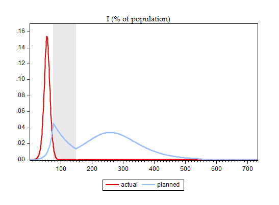
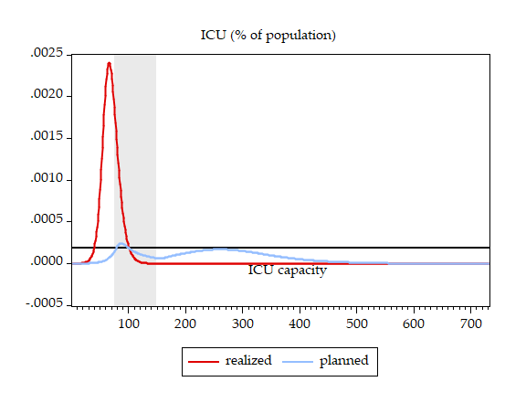
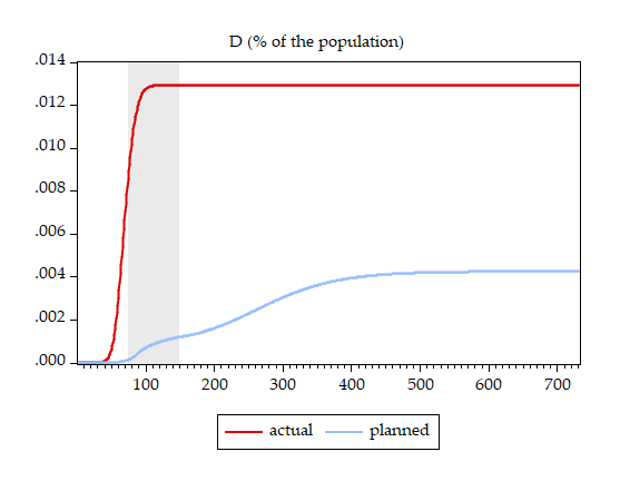
To illustrate, and to work within a realistic setup, we let the policymaker decide on when to start and when to stop a lockdown (see Bar-On et al. 2020a for details and Alon et al. 2020 for a richer analysis of the policymaker’s problem). We assume that the policymaker relies on the erroneous SIR specification. We derive the optimal lockdown timing, which turns out to be `lockdown on day 75 and release on day 147,’ and subsequently compare the results under two scenarios: (i) the disease behaves according to the perception of the policymaker (denoted ‘planned’) and (ii) the disease behaves according to the epidemiologically-grounded full model (denoted ‘realised’). Figure 3 presents the results, comparing ‘planned’ and ‘realised’ disease scale, deaths, and ICU patients.
Figure 3 Disease dynamics
Panel a
Panel b
Panel c
Notes: Lockdown period is shaded.
One can immediately see the price of basing the optimal policy design on an assumed slow-moving disease while in fact dealing with a fast-moving disease:
(i) The planned lockdown comes too late – after the peak has passed and the bulk of deaths has already occurred;
(ii) The planned lockdown was supposed to induce a very small breach of ICU capacity, spreading peak ICU demand over two moderate waves, whereas realised ICU demand soars, breaching capacity more than ten-fold while the policymaker still waits and does nothing;
(iii) Actual deaths are three-times higher than planned – 4.28 million people in the US case.
Regarding the numbers of deceased in this analysis, in Alon et al. (2020), we show that much more favourable outcomes with much lower death numbers can be attained when the policymaker has more choices of lockdown strategies. The cost of misspecification, though, remains high.
Furthermore, in the real world, US deaths are currently almost 160,000, an order of magnitude lower than even the relatively `benign’ first scenario above. This is because US policymakers have imposed longer lockdowns than the hypothetical policymaker above, as they have access to wider policy choices.
Finally, most papers that use the SIR model present even higher numbers of deaths, in the order of magnitude of the second scenario above or worse.
Summing up
There is a tremendous cost in lives lost that is generated by policy based on a misperception of the disease dynamics.
We conclude that of all misspecifications, the gravest inaccuracy in disease dynamics is made by those who posit that the infectious period and disease duration till death are identical. Other types of misspecification, such as ignoring the latent stage or not considering sub-compartments, are of smaller magnitude.
We also discuss errors in modelling lockdowns in light of the above. For example, we show that the quadratic matching properties of the model, flagged by economists, holds only in highly unrealistic and implausible lockdown situations.
References
Alon, Uri, Tanya Baron, Yinon Bar-On, Ofer Cornfeld, Ron Milo and Eran Yashiv (2020), “COVID-19: Looking for the exit“, working paper.
Bar-On, Yinon, Tanya Baron, Ofer Cornfeld, Ron Milo and Eran Yashiv (2020a), “Caveats for economists: Epidemiology-based modelling of COVID 19 and model misspecifications”, CEPR Discussion Paper 15107.
Bar-On, Yinon, Ron Sender, Avi Flamholz, Rob Phillips and Ron Milo (2020b), “A quantitative compendium of COVID-19 epidemiology”, arXiv:2006.01283.
Kermack, William O, and Anderson G McKendrick (1927), “A contribution to the mathematical theory of epidemics,” Proceedings of the Royal Society London Ser. A, 115: 700–21.
Endnotes
1 Not to be confused with the incubation period, which is the time it takes from infection to the onset of symptoms.
2 Following experimentation, we adopt the specification of two sub-compartments. The latent and infectious periods are the sum of the time spent in the E₁ and E₂ or I₁ and I₂ sub-compartments, respectively, and their distribution is thus the same as that of a sum of exponentially distributed random variables. The latter distribution is known as the Erlang distribution, and this type of augmented model is known as the SEIR-Erlang model.
3 In formal terms R = b/g and a long infectious period means a low value for g and thus a low value for the disease transmission parameter b, given a value of the reproduction parameter R.
4 See Bar-On et al. (2020a) for full details of the parameterisation.
5 Or the exposed and infectious, in models that include the latent stage.


