A good understanding of the Phillips curve-type mechanism has always been an important ingredient for the conduct of monetary policy. This fundamental relation between the real and the nominal side of the economy provides a useful gauge of past and future inflationary dynamics. The steepness of the Phillips curve matters: the flatter the Phillips curve, the higher the inflation stabilisation costs that central banks face in terms of employment and real activity. In the abnormal times of the COVID-19 pandemic this is even more relevant, as the uncertainty related to future inflation developments is particularly high. Some believe that deployed expansionary policies and ensuing pent-up demand will lead to higher inflation (Summers 2021), while others believe that consumers might become more cautious, depressing demand for longer. Irrespective of the scenario one subscribes to, the steepness of the Phillips curve matters for the impact on inflation (Krugman 2021).
Understanding the Phillips curve relationship was challenging even before the pandemic, with many economists (in particular, for the US case) arguing that the relationship is dead and that other factors apart from slack matter for inflation. Such factors include globalisation, inflation expectations and some even argue that inflation follows a pure exogenous process. High uncertainty resides also in the way that certain states of the economy affect this relation, with no consensus to date on the strength or shape of possible non-linearities. At the same time, there is evidence that headline inflation is increasingly ‘determined abroad’, whereas core and wage inflation are still considered to be largely a domestic process (Forbes 2019).
For the euro area there is a broad consensus that both price and wage Phillips curves are still alive, though admittedly not very steep. Recent studies approach the Phillips curve within a so-called thick modelling framework, whereby a comprehensive set of inflation drivers is considered to understand inflation dynamics. This is a powerful way to hedge against model uncertainty (see Ciccarelli and Osbat 2017 and Moretti et al. 2019 for price inflation, and Nickel et al. 2019 for wage inflation). Moreover, Ball and Mazumder (2021) show that when core inflation is measured as the weighted median of industry inflation rates, then economic slack explains a larger share of euro area inflation. This relationship plays an important role in the analysis of the economic outlook and the formulation of monetary policy at the ECB (Eser et al. 2020) and also in communicating to the public about inflation (Schnabel 2021).
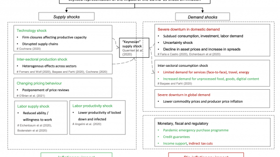
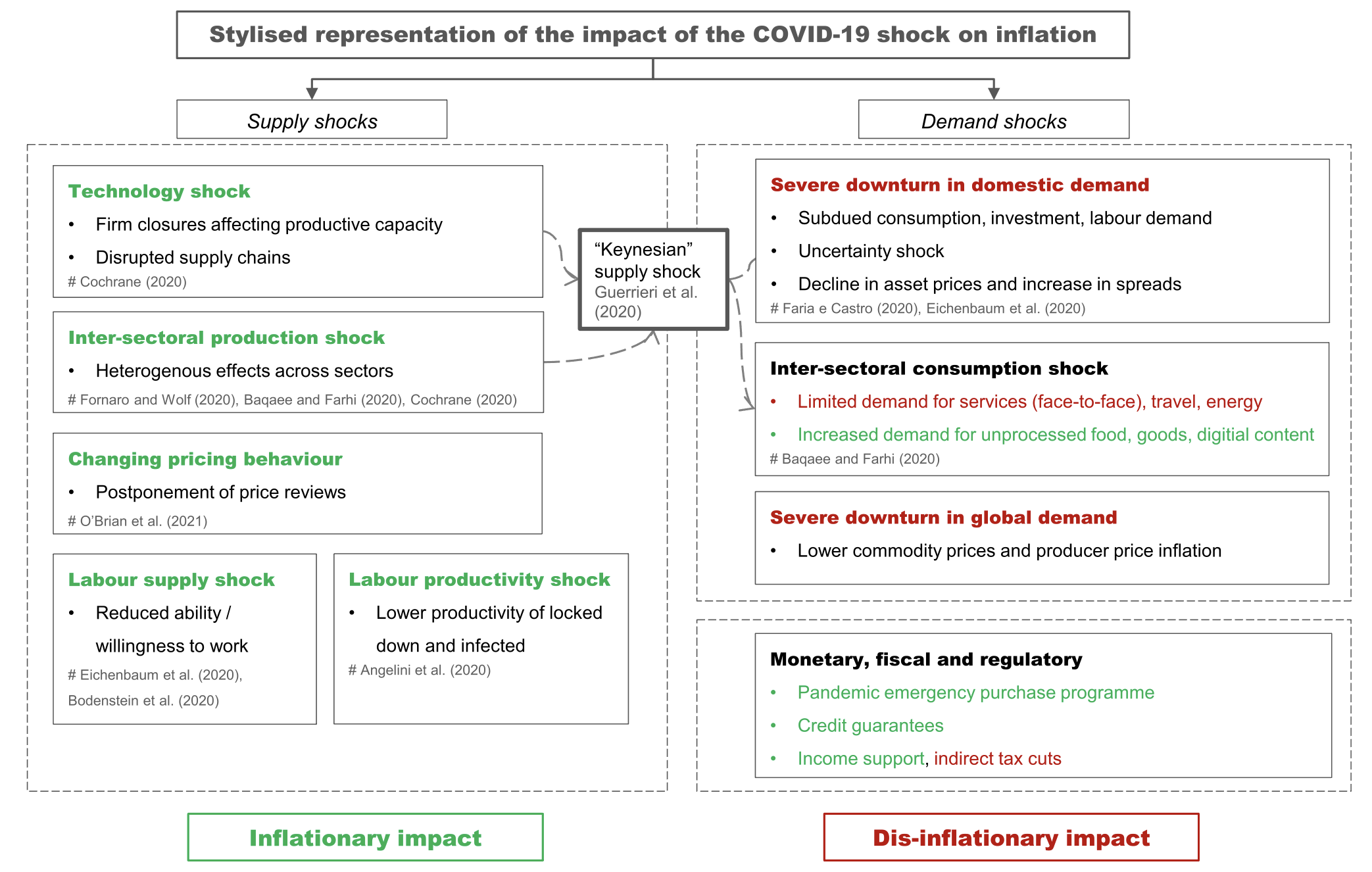
The pandemic calls for a careful interpretation of this established relationship because this episode differs dramatically from a ‘usual shock’ – both in composition and in size. In terms of composition, it encompasses complex and interrelated supply and demand channels, domestic and external forces, unprecedented policy responses, as well as highly heterogenous effects across sectors and agents. Figure 1 provides a stylised representation of various channels through which the COVID-19 shock initially affected inflation. Initially, the COVID-19 pandemic manifested itself as supply shocks related to lockdowns and firm closures. This blurs the Phillips curve relation as it moves prices and activity in opposite direction. At the same time, it also triggered a series of demand shocks due to the increased uncertainty about lockdown measures and the risk of infection. The distinction between supply and demand effects then quickly became even more obscured as consumers adapted and changes in supply triggered demand effects (Guerrieri et al. 2020). In addition, demand shifts likely triggered supply-side frictions, whereby increased demand for some goods created inflationary pressures in sectors trying to build capacity. Apart from that, unprecedented policy responses blur the observed economic outcomes and relationships. All in all, observed prices and output reflected not only demand shocks, which trigger the theoretical positive co-movement between prices and output, but also larger than usual supply shocks and policy shocks which can lead to apparent Phillips curve flattening (Tenreyro and McLeay 2019).
Figure 1 Complex effects of the COVID-19 shock on inflation
Note: The constellation of shocks hitting the economy is changing as the recovery progresses
Source: Adapted from Bobeica and Hartwig (2021).
In terms of its size, the COVID-19 shock wreaked havoc on conventional time series models, including standard Phillips curves. In a recent paper we show that when adding only 3 COVID-19 observations to a sizeable euro area sample, the estimated parameters of the Phillips curve for HICP excluding energy and food change markedly, see Figure 2. This result is robust for a battery of Phillips curve models within a thick modelling approach. The Phillips curve appears to flatten across all considered slack measures; the absolute change in coefficients is small, but given that the Phillips curve was rather flat before COVID-19, the slope diminishes by around 40 to 50 percent for some specifications. We argue that it is too soon to ascertain structural changes. Rather than taking this change at face value, this points to a limitation of Gaussian models to cope with extreme shocks.
Figure 2 Change in Phillips curve parameters after adding three quarters (2020Q1-Q3) to the sample (comparison of sample ending in 2020Q3 vs. in 2019Q4)
Note: Each bar corresponds to one Phillips curve specification of a fixed parameter regression model with various measures of slack: GDP growth, unemployment rate (UR), output gap and unemployment gap (U gap). 1,2,..,10 indicate specifications with various measures of expectations, in the following order: 1 - 6 are Consensus 1,2,..,6 quarters ahead, 7 - 9 are SPF 1,2,5 years ahead, 10 - no expectation term. No intercept was included in the specification with SPF 5 years ahead. For the unemployment rate and gap the change in slope refers to coefficients with reversed sign.
Source: Bobeica and Hartwig (2021).
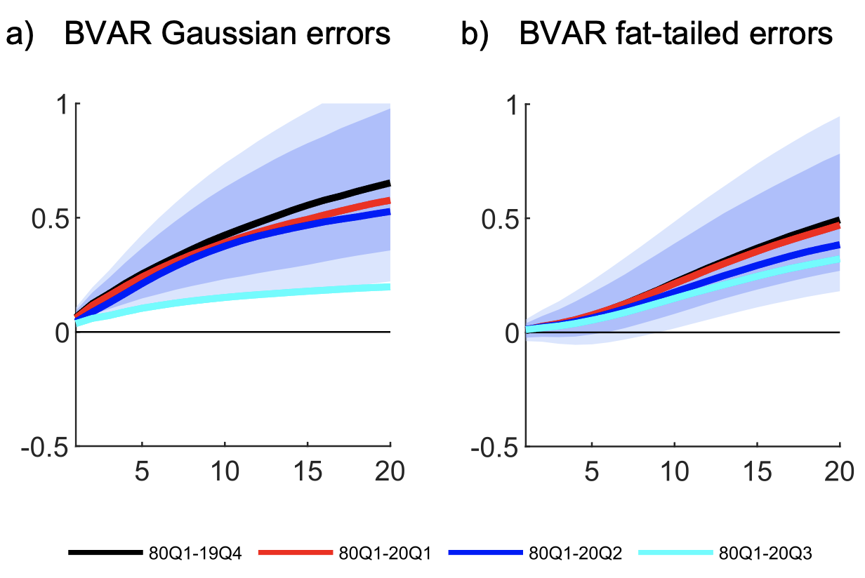
There are by now several econometric solutions on how to adjust standard time series models to deal with the abnormal variations in the data. What they have in common is that they suggest down-weighing the impact of the COVID-19 observations to diminish the impact on established economic relationships (such modelling solutions were proposed, for instance, by Lenza and Primiceri 2020 and Carriero et al. 2021). Bobeica and Hartwig (2021) show that allowing the errors of a Bayesian vector autoregression (VAR) to have a heavy-tailed error distribution instead of a Gaussian one is a sufficient extension to ensure stable parameters. Intuitively, fatter tails allow the abnormal observations to be soaked up by residuals rather than distorting coefficients. This solution is simple and appears to characterise the data well even before the COVID-19 pandemic. It is worth noting that multi-equation models like VARs are better equipped than single-equation models like Phillips curves to deal with the impact of abnormal observations, where the same extensions are less effective. Figure 3 shows that the estimated link between inflation and real activity is more stable in a model with heavy-tailed errors compared to a Gaussian one. Specifically, the response of inflation to a shock in real GDP drastically flattens with the impact of the COVID-19 observations in a standard Bayesian VAR with Gaussian errors (black versus cyan line), while under heavy-tailed errors these changes are more limited.
Figure 3 Response of inflation to a shock in real GDP
Note: Thick lines are median estimates and the dark (light) blue area is the 68% (90%) credible interval for the estimation window until 19Q4.
Source: Bobeica and Hartwig (2021)
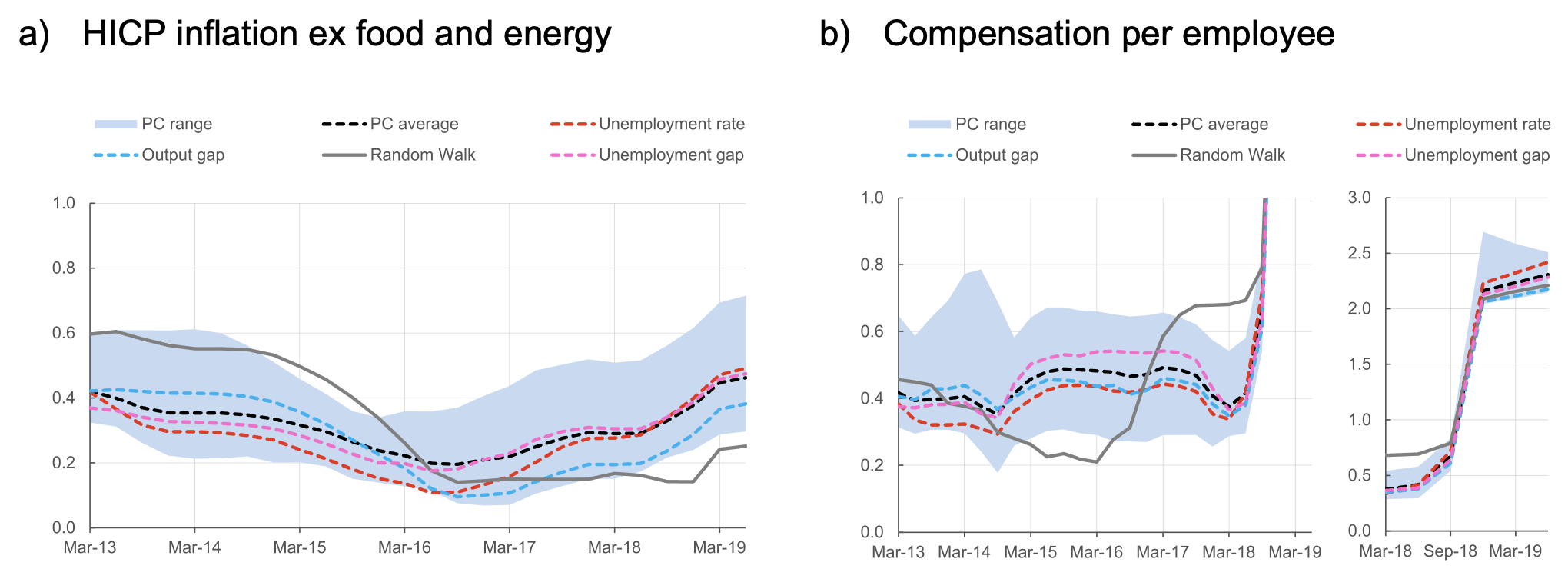
The massive impact of the COVID-19 shock is also reflected in a break in the ability to forecast price and wage inflation. Figure 4 illustrates the results of a real-time conditional forecast evaluation using hybrid Phillips curve models for both price and wage inflation. As already documented in the literature, the forecast performance of Phillips curve models varies significantly over time. For price inflation, Phillips curve models post a deterioration in their forecasting performance relative to the random walk over the last couple of years, which continued over the COVID-19 crisis (last observations in the chart).
The compensation per employee measure was heavily distorted during the COVID-19 pandemic by short-time work and temporary lay-offs in the context of job retention schemes. No forecasting model could have predicted what unprecedented labour market measures could do to wage inflation. Unsurprisingly, the ability to forecast wage inflation was even more severely hampered when comparing to price inflation. Nevertheless, it is worth pointing out that before the pandemic euro area wage inflation was better predicted by Phillips curves models than by a random walk.
Figure 4 RMSFE for two-year ahead forecast in a real-time forecast evaluation (three-year moving average)
Note: PC range stands for the range covering all Phillips curve forecasts. The dotted lines show the average per slack across all considered expectation measures of fixed and time-varying parameter regression models. Forecasts are obtained conditional on the future path of the slack measures, imported inflation (price PC only) and productivity (wage PC only) as projected within the European (System of) Central Banks Broad Macroeconomic Projection Exercises. For expectations, an autoregressive process is used.
Before COVID-19, wage inflation was more responsive to developments in the real economy as compared to price inflation. The validity of the euro area wage Phillips curve has been ascertained in Nickel et al. (2019) for various wage inflation measures. Figure 5 shows the estimated Phillips curve slope in real time, using the information set that a researcher would have had at her disposal in each given quarter. The stronger cyclical sensitivity of wage growth as compared to prices holds also after controlling for the fact that compensation per employee is more volatile than underlying inflation. However, for both inflation measures the link with unemployment (particularly with a conventional unemployment gap) has been somewhat weakening over time, pointing towards the difficulties in measuring slack in the labour market. These difficulties have dramatically increased during the pandemic and the high uncertainty surrounding the measurement of slack is another argument calling for caution when assessing changes in the slope of the Phillips curve for both wage and price inflation at the current juncture.
Figure 5 Slope of Phillips curve in real time (averages per slack across all specifications)
Note: The x-axis shows the end of the estimation sample starting in 1995. Averages per slack across all specifications with various inflation expectation measures of fixed and time-varying parameter regression models. Inverted slope for unemployment rate and unemployment gap.
Distortions in official statistics for both price and wage inflation are another factor that complicate the assessment on the slope of the Phillips curve after the COVID-19 shock. In the case of price inflation, official statistics are partly affected by numerous temporary and technical factors, unrelated to developments in real activity (e.g. swings in the energy component, a sizable share of imputed prices, changes in indirect taxes in some member state, changes in the timing and scope of seasonal sales, abnormal variations in expenditures weights). In the case of wage inflation, sizeable data distortions are induced by the coronavirus support policies (e.g. job retention schemes, government transfers). On top, the aggregate data conceals sizeable compositional effects, as employment declined particularly strong for certain categories, such as low-skilled and young workers.
While a formal quantitative assessment of the slope/shape of the Phillips curve during the pandemic is hindered by a myriad of technical and economic factors, there is evidence pointing towards the conclusion that the Phillips curve-type mechanism is still at play. Underlying inflationary pressures in the euro area have been dampened by the build-up of economic slack. After an initial stickiness, HICP inflation excluding energy and food reached 0.2% at end-2020, suggesting that the link with the amount of slack is playing a role. Also, while at the beginning of the pandemic the constellation of shocks blurred Phillips curve relations (supply shocks dominated), the normalisation phase is characterised by demand shocks kicking in and re-establishing the positive relation between prices and real activity. Supportive evidence for the link between prices and demand is provided also by micro data. Web-scraped supermarket data from PriceStats for the big-five euro area countries revealed that the textbook relation between prices and demand is not dead. The number of products available online started to decrease at the beginning of March 2020 and, at the same time, the share of products offered at a discount was nearly 40% lower in mid-April 2020 than a year earlier (Henkel et al. Rodari 2021). On the wage inflation side, where the data distortions are even more pronounced, there is some indication that the higher slack in the labour market might play a role. Wage negotiations during the pandemic have been delayed or, for a few countries where such negotiations have been concluded, the outcome points to lower wage increases (in some cases, no increases).
To conclude, the pandemic made it even more obvious that “finding the Phillips curve is like finding a needle in a haystack. But it is hidden there somewhere!” (Reichlin 2018).
Authors’ note: The views expressed are the authors and do not necessarily reflect those of the ECB.
References
Ball, L and S Mazumder (2021), “A Phillips curve for the euro area”, International Finance 2-17.
Bobeica, E and B Hartwig (2021), “The COVID-19 shock and challenges for time series models”, ECB Working Paper 2558.
Carriero, A, T E Clark, M Marcellino and E Mertens (2021), “Addressing COVID-19 Outliers in BVARs with Stochastic Volatility”, Federal Reserve Bank of Cleveland Working Paper.
Ciccarelli, M and C Osbat (2017), "Low inflation in the euro area: Causes and consequences", ECB Occasional Paper 181.
Eser, F, P Karadi, P R Lane, L Moretti and C Osbat (2020), “The Phillips Curve at the ECB”, The Manchester School 88: 50-85.
Forbes, K (2019), “Inflation dynamics: Dead, dormant, or determined abroad?”, NBER Working Paper 26496.
Guerrieri, V, G Lorenzoni, L Straub and I Werning (2020), “Macroeconomic Implications of COVID-19: Can Negative Supply Shocks Cause Demand Shortages?”, NBER Working Paper 26918.
Henkel, L, A Lentini and F Rodari (2021), "The role of microdata in inflation analysis", ECB Economic Bulletin.
Krugman, P (2021), “Stagflation revisited. Did we get the whole macro story wrong?”, Substack, 05 February.
Lenza, M and G Primiceri (2020), “How to Estimate a VAR after March 2020”, NBER Working Paper 27771.
Moretti, L, L Onorante and S Z Saber (2019), “Phillips curves in the euro area”, ECB Working Paper 2295.
Nickel, C, E Bobeica, G Koester, E Lis and M Porqueddu (2019), “Understanding low wage growth in the euro area and European countries”, ECB Occasional Paper 232.
Reichlin, L (2018), “Discussion of slack and cyclically sensitive inflation by Stock and Watson”, Sintra: ECB Annual Forum.
Schnabel, I (2021), “Escaping low inflation?”, Speech by Isabel Schnabel, Member of the Executive Board of the ECB, at the Petersberger Sommerdialog.
Summers, L H (2021), “The Biden stimulus is admirably ambitious. But it brings some big risks, too”, The Washington Post, 04 February.
Tenreyro, S and M McLeay (2019), "Optimal Inflation and the Identification of the Phillips Curve", NBER Macroeconomics Annual 34: 199-255.
