Covid-19 has caused an economic crisis that is remarkable for its disparate effects. Some sectors are booming – manufacturers, for instance, have struggled to keep up with demand for new cars.1 Meanwhile, no other economic crisis, not even the Great Depression, can compare with the current moment for distress in the food services and accommodations sector.2
The differential impact across sectors has led to a ‘K-shaped’ recovery in which high-education, high-income workers do relatively well, while workers with less education are hard hit. Workers without a college degree are more likely to do in-person work in businesses such as restaurants for which demand has fallen. Workers with a college a degree, by contrast, can often do their jobs remotely. Between February and October 2020, employment of workers with less than a high school degree fell 9%; that of workers with a bachelor’s degree fell just 3%.3 Initially, the household income effects of these differential employment trends were blunted by the additional $600 per week in unemployment insurance payments authorised by the CARES act. Since the end of these additional payments in July, the difference in employment trajectories may now translate into differences in income trajectories, a pattern reinforced by the effect of higher stock and housing prices on capital gains income for those at the top end of the income distribution.
Such inequality is both important in and of itself and may matter for the future aggregate behaviour of the economy, since workers in different sectors and with different education and income levels have different marginal propensities to consume. There is a recent and rapidly growing literature on the ways in which the distributional effects of shocks impact the aggregate economy (e.g. Auclert 2019, Cloyne et al. 2020). In a recent paper (Hausman et al. 2020), we contribute to this literature by examining how a shift in income away from farmers in the US changed the course of the Great Depression. The analogue to the current recession is not direct, but our paper shows how studying the distributional effects of a shock can help one to understand the aggregate behaviour of the economy.
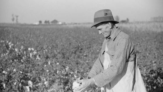
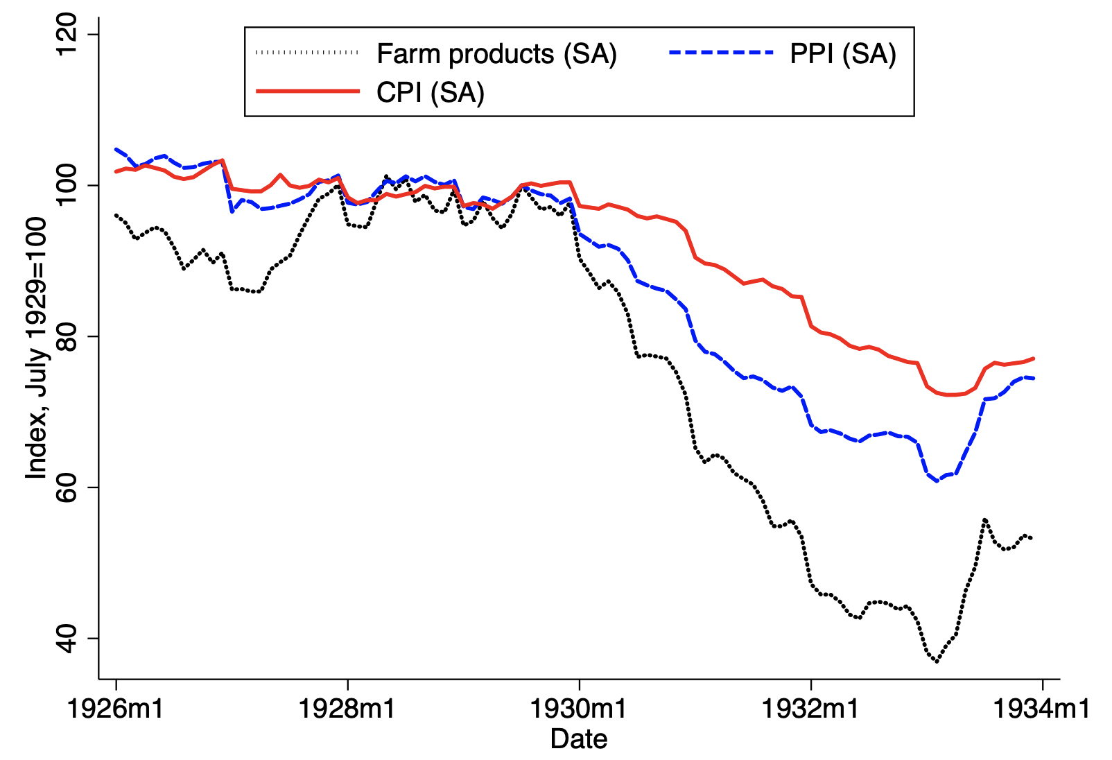
When the Great Depression began in 1929, farmers made up roughly 25% of the population.4 Many more people lived in small towns whose economies depended on demand from nearby farmers. Unfortunately for farmers and their neighbours, when the world economy fell into a deep recession in 1930, farm product prices collapsed. The seasonally adjusted price of cotton, for instance, fell 39% between the fourth quarter of 1929 and the third quarter of 1930. Figure 1 illustrates that farm product prices as a whole fell much more rapidly during the Great Depression than did other producer prices or the CPI. The decline in farm product prices was likely the result of a decline in demand combined with an inelastic supply.
Figure 1
Note: The figure shows the level of seasonally adjusted farm product prices, producer prices (PPI) and consumer prices (CPI). For sources and seasonal adjustment details, see the note to Figure 2 in Hausman et al. (2020).
For a farmer at the time, declines in the price of their product translated directly into declines in their household income. Thus between 1929 and 1930, real (CPI-deflated) nonfarm income fell 6% while real farm income fell 25%. As some contemporaries recognised, this lent a sort of downward angled K-shape to the Great Depression – while no sector prospered, farmers did worse than nonfarm households. The American economist Irving Fisher wrote, for instance, that “[t]he evils of deflation and liquidation through bankruptcy and default manifest themselves more malevolently in agriculture than in any other great industrial group” (Fisher 1932: 32).
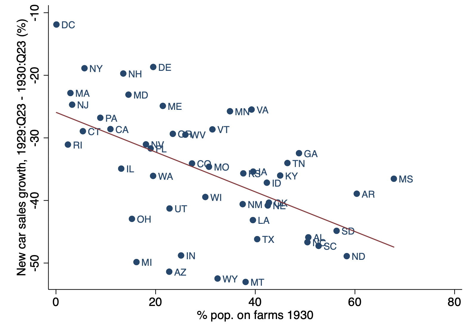
In our paper, we study the effect of the decline in farm product prices in 1929-30, the first year of the Great Depression. Using auto sales data by state and by county in Ohio, we find that the large decline in farm product prices and incomes led to a collapse of spending in farm areas. We use auto sales (specifically, new passenger car registrations), since they are well-measured and are likely correlated with other types of consumption. Figure 2 shows the relationship between the percent of a states’ population living on farms in 1930 and the percent change in car sales in the first year of the Great Depression. There is a clear negative relationship, with the farm share of the population explaining almost a third of the cross-state variation in auto sales. The slope coefficient (-0.32) implies that a one standard deviation change in farm population share (17 percentage points) is associated with 5.5 percentage points more negative auto sales growth. This relationship is robust to controlling for region fixed effects, drought, total state population, and pre-depression car sales.
Figure 2
Note: The percent change in car sales is measured between the six-month average of car sales in the second and third quarter of 1929 and the six-month average of car sales in the second and third quarter of 1930. For sources, see Hausman et al. (2020).
To learn more about the sources of large consumption declines in farm areas, we look at what sort of agricultural activity was most associated with lower auto sales in 1930. We find that it was traded crop production rather than agricultural production as a whole. This is consistent with larger declines in the prices of traded crops (e.g. cotton and wheat) than in the prices of nontraded farm products (e.g. milk and hay). This result – that more negative auto sales growth was associated with traded crop production and not with non-traded farm product production – is supported by county-level auto sales data from Ohio.
Lower farm product prices were bad for farmers but good for the businesses and workers that consumed farm products. The incidence of this benefit depended on the degree to which lower farm product prices were passed through to final goods prices. The prices of many final goods were sticky, so lower farm product prices benefited manufacturers, not just final consumers. For example, the producer price of tobacco fell 23% from 1929-30, but the price of a pack of cigarettes rose 2%.
The aggregate impact of lower farm product prices depended on the relative marginal propensity to consume of the households and businesses losing and gaining from the price change. We argue that farmers likely had a higher marginal propensity to consume than the businesses and workers who gained from lower farm product prices. Farmers in 1929 are the analogue of mortgaged US households in 2008 – they had large debt burdens that made maintaining consumption difficult when income declined. In 1930, farm mortgage debt was 190% of net farm personal income, while residential mortgage debt was 39% of nonfarm personal income. We have three reasons to believe that farmers’ debt burden led to a large spending response to the decline in farm product prices. First, this is predicted by theory. Second, in Hausman et al. (2019) we find that in 1933, an increase in farm product prices increased auto sales more in counties where more farms were mortgaged. Third, in the 2008 financial crisis more leverage was associated with larger declines in household consumption (Mian et al. 2013).
Farmers’ relatively high marginal propensity to consume meant lower farm product prices had negative aggregate effects; farmers responded to lower incomes by curtailing their spending. Businesses and workers responded to their gain from lower farm product prices with smaller spending increases. To obtain a quantitative sense of how large an aggregate effect lower farm product prices might have had, we use a model-based calculation developed in Hausman et al. (2019). With assumptions about the pass-through of farm product price changes to workers, the relative marginal propensity to consume of farmers, businesses, and workers, and the aggregate multiplier, we can translate our cross-state regression coefficient into an estimate of the aggregate impact of lower farm product prices. A plausible range of parameters suggests that the decline in farm product prices explains 10-30% of the decline in US output before October 1930.
Just as a collapse of farm area consumption was part of what made the Great Depression so severe, its recovery helped end the depression. In Hausman et al. (2019), we show that Franklin Roosevelt’s decision to take the US off the Gold Standard in April 1933 led to a large increase in the real price of traded farm products. This in turn drove a remarkably rapid recovery of the entire US economy (see also Temin and Wigmore 1990).
The current economic crisis caused by the coronavirus is unique; direct lessons from history are difficult. It would be a mistake, for instance, to try to increase demand for the most hard-hit sectors now. The UK made a mistake when it subsidised eating at restaurants in August 2020; Fetzer (2020) shows that this policy led to many coronavirus clusters with resulting large public health and economic costs. Still, the idea of directly helping workers in the hardest-hit sectors may have relevance to current policy. If the workers most affected by the economic crisis have relatively high marginal propensities to consume, it may be good aggregate macro policy, as well as good social policy, to provide relief payments to these workers.
References
Auclert, A (2019), “Monetary Policy and the Redistribution Channel”, American Economic Review 109(6): 2333-2367.
Cloyne, J, C Ferreira, and P Surico (2020) “Monetary Policy when Households Have Debt: New Evidence on the Transmission Mechanism”, Review of Economic Studies 87(1): 102-129.
Fetzer, T (2020), “Subsidizing the Spread of COVID19: Evidence from the UK’s Eat-Out-to-Help-Out Scheme”, CAGE Working paper no. 517.
Fisher, I (1932), Booms and Depressions: Some First Principles, Adelphi.
Hausman, J K, P W Rhode, and J F Wieland (2019), “Recovery from the Great Depression: The Farm Channel in Spring 1933”, American Economic Review 109(2): 427-472.
Hausman, J K, P W Rhode, and J F Wieland (2020), “Farm Product Prices, Redistribution, and the Early U.S. Great Depression”, NBER Working Paper 28055.
Mian, A, K Rao, and A Sufi (2013), “Household Balance Sheets, Consumption, and the Economic Slump”, Quarterly Journal of Economics 128(4): 1687-1726.
Temin, P and B A Wigmore (1990), “The End of One Big Deflation”, Explorations in Economic History 27: 483-502.
Endnotes
1 https://www.wsj.com/articles/factories-hum-to-keep-up-with-auto-housing-demand-11603816320.
2 Between the fourth quarter of 2019 and the third quarter of 2020, real consumption expenditure on food services and accommodations fell 19%; between 1929 and 1933, expenditure in this category fell 6% (NIPA table 2.3.3).
3 Bureau of Labor Statistics, Household Data, Table A-5. For more description of these patterns, and the differential recovery trends by education and income, see https://www.wsj.com/articles/the-covid-economy-carves-deep-divide-between-haves-and-have-nots-11601910595.
3 Unless otherwise noted, all facts that follow come from Hausman et al. (2020).


