Mortgage markets are widely believed to play an important role in driving business cycles (Iacoviello and Neri 2010). Moreover, there is increasing evidence that the housing cycle and mortgage market design affect the working of monetary policy. For instance, Calza et al. (2013) show that monetary policy is more powerful when mortgages are of a variable-rate type, while Jordà et al. (2020) present evidence that mortgage credit growth amplifies monetary restraint.
The mortgage market features that make the monetary policy reaction dependent on the phase of the housing cycle are highly non-linear. First, collateral constraints bind only occasionally – when house prices are low, many households can face a binding constraint when trying to take a loan. However, when house prices are soaring, the value of collateral can often be higher than what is required by banks for given loan demand. As nobody can be forced to take a loan only because he or she has sufficient collateral, the collateral constraint becomes slack. Second, a bank can decide to grant fewer loans when it wants to de-leverage, but it usually cannot force people already holding long-term debt to accelerate their repayments. In other words, new loan originations can decline sharply (even to zero), but cannot become negative.
Incorporating realistic features of the mortgage markets into a quantitative macroeconomic model is challenging from a technical point of view, despite important progress having been made, among others, by Justiniano et al. (2015), Guerrieri and Iacoviello (2017), and Garriga et al. (2017). This column is based on our recent paper (Bluwstein et al. 2020), where these technical difficulties have been resolved. In particular, we successfully estimate a structural macroeconomic model that includes both non-linearities mentioned above.
Phases of the housing cycle
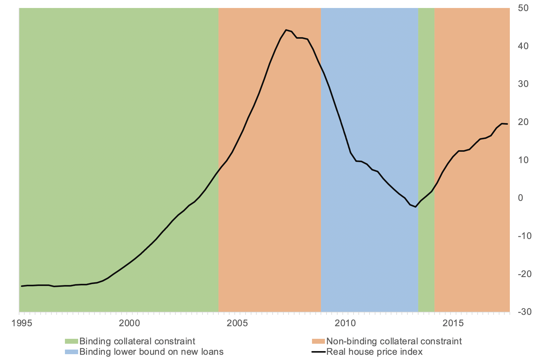
A key advantage of having an estimated structural model is that it allows us to offer a quantitative analysis of the housing market-related non-linearities and their relevance for the transmission of monetary policy. Figure 1 presents the identified phases of the housing cycle for the US economy, plotted against the real house price index.
Figure 1 Housing market regimes
As house prices in the US were relatively depressed after the 1990/91 recession, collateral value was low and households were largely constrained in their borrowing. According to our model, this changed around 2004, when the collateral constraint stopped binding and households taking new loans were borrowing less than they actually could. When the Great Recession hit the US economy, house prices began to fall. Around 2009 they were falling sharply enough to trigger the second constraint, which effectively prevented lenders from de-leveraging as fast as they would have liked to. A rebound in house prices that started at the end of 2013 activated the collateral constraint again, but not for long. As house prices did not fall all the way to the levels observed in the early 2000s, their quick recovery made the credit constraint non-binding by mid-2014.
Implications for monetary policy effectiveness
What do these different identified regimes mean for the effectiveness of monetary policy? According to our analysis for the US, they make it state dependent.
We illustrate this in Figure 2, which plots the response of household mortgage debt and output to a typical monetary easing at three selected dates. The first one comes from the mid-1990s, when the collateral constraint was binding. As a fall in central bank rates pushes up house prices (and hence the value of collateral), households can borrow more, which eventually leads to an increase in aggregate demand and output. The second date we pick is the mature phase of the house price cycle in 2006, when the collateral constraint was slack. As lower interest rates constitute a positive income shock for borrowers, they actually decrease their debt in line with the standard consumption smoothing motive. As the financial accelerator is not active, output growth is smaller for the same scale of monetary stimulus. Our final date is 2010, when house prices were falling sharply, and de-leveraging was limited by a constraint that prevents lenders from imposing an acceleration of debt repayment. In these circumstances, a monetary stimulus does not have any significant effect on credit. As a result, the reaction of output is also dampened compared to the situation in 1995.
Figure 2 Regime-dependence in the effects of monetary policy tightening
Asymmetries in monetary transmission
The non-linearities that we capture in our framework also imply that the effects of monetary policy might exhibit strong asymmetries.
Figure 3 plots the responses to positive and negative monetary shocks at the beginning of 2002, which is when the collateral constraint was still binding (but new loans were very close to their lower bound). As can be seen from the first row, monetary easing leads to an expansion in debt and output that is very similar to that obtained for 1995Q1 in Figure 2. In contrast, as depicted in the second row, after an increase in the policy rate, new loans hit the lower bound, which effectively limits their adjustment for the first two periods after the shock. As a result, debt responds with a delay, and so does output, reaching its trough only after a year (rather than on impact).
Figure 3 Asymmetric effects of monetary tightening and easing
Tough luck in bad times?
The key takeaway from this column is that monetary easing in the US has been less efficient when house prices were high or started falling rapidly. This is relevant in the current context, when policy makers have to respond to the Covid-19 pandemic, at a time when residential property valuations are high in many advanced economies. More generally, our findings give additional support to the view that the housing market should be closely monitored by the monetary authorities, especially since its phases are not perfectly synchronised with the business cycle. In particular, for the central bank’s potency to fight a recession, it may matter whether the economy enters it with high or low house prices.
References
Bluwstein, K, M Brzoza-Brzezina, P Gelain and M Kolasa (2020), "Multiperiod Loans, Occasionally Binding Constraints, and Monetary Policy: A Quantitative Evaluation", Journal of Money, Credit and Banking 52(7): 1691-1718.
Garriga, C, F E Kydland and R Šustek (2017), “Mortgages and Monetary Policy”, Review of Financial Studies 30: 3337-3375.
Guerrieri, L and M Iacoviello (2017), “Collateral Constraints and Macroeconomic Asymmetries”, Journal of Monetary Economics 90: 28-49.
Iacoviello, M and S Neri (2010), “Housing Market Spillovers: Evidence from an Estimated DSGE Model”, American Economic Journal: Macroeconomics 2(2): 125-164.
Jordà, Ò, M Schularick and A Taylor (2020), “The effects of quasi-random monetary experiments”, Journal of Monetary Economics 112: 22-40.
Justiniano, A, G E Primiceri and A Tambalotti (2015), “Household Leveraging and Deleveraging”, Review of Economic Dynamics 18: 3-20.


