The Great Recession reached the US in December 2007. In 2008, unemployment rose rapidly, and in response the Fed swiftly cut interest rates. In December 2008, however, monetary policy ran out of fuel. The nominal interest rate had reached the zero lower bound, prompting the US government to look for alternative stabilisation policies. One policy that had been used before and was considered again, was to increase public expenditure through a stimulus package – the American Recovery and Reinvestment Act, described by Romer and Bernstein (2009).
As policymakers and academic researchers started to discuss what the appropriate amount of stimulus spending should be, the lack of consensus became evident. A number of arguments were advanced in favour of and against the stimulus package. These arguments often involved the ‘output multiplier’, which is the increase in GDP achieved by a one-dollar increase in public expenditure. A positive multiplier means that an increase in public expenditure raises GDP. A multiplier larger than one means that an increase in public expenditure raises GDP more than one-for-one, implying that the increase in public expenditure raises other components of GDP – such as household consumption.
One part of the debate was about the size of the multiplier, and especially whether it was bigger or smaller than one. Some argued that the stimulus package was justified because the multiplier was bigger than one. Others retorted that the multiplier was smaller than one and hence the stimulus package was a bad idea. More generally, a lot of the debate was guided by the ‘bang for the buck’ approach – the larger the multiplier, the more effective the policy, and therefore the more it should be used.
Another part of the debate revolved around the usefulness of public expenditure. A concern of stimulus sceptics was that additional public expenditure may not be very useful. In the worst case, we would build bridges to nowhere, but even in a less dire view, public spending would not be as socially valuable as private spending.
In recent work (Michaillat and Saez 2019), we study the design of stimulus packages at the onset of recessions. We aim to revisit these arguments and offer a blueprint for when the next stimulus package will be needed. As most modern research on business-cycle stabilisation has focused on monetary policy, not much is known about the properties of an adequate stimulus package. Indeed, because the Federal Reserve has been in charge of stabilisation for several decades, the design of optimal monetary policy has attracted an enormous amount of research, while the design of optimal stimulus packages has been relatively neglected.
Before we discuss the properties of a well-designed stimulus package, let us say a few words about the model we use for the analysis. We built a model that captures all the elements that played a prevalent role in the policy debate. Although experts may disagree on the exact values that each of the relevant statistics take, what we think might be helpful at the very least is a coherent framework in which all these different values can be plugged in.
Our model features unemployment, which may be at the right level or inefficiently high, as in recessions. We allow public expenditure to be anything from useless to as useful as private expenditure. The value of public expenditure is described by an ‘elasticity of substitution between public and private consumption’. This elasticity describes the utility derived from additional public goods – with zero elasticity, extra public goods are useless. A higher elasticity means that extra public goods are more valuable, and with infinite elasticity, public and private goods are interchangeable. We also allow public spending to be anything from totally ineffective to very effective at stimulating GDP and reducing unemployment. The effectiveness of public spending is measured by the output multiplier, which in our model is allowed to be negative, zero, below one, or above one.
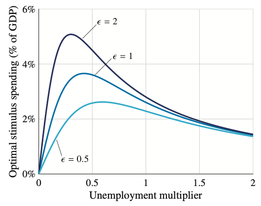
Several properties of a well-designed stimulus package stand out – because they challenge existing preconceptions. The first is that the size of the stimulus does not follow the bang-for-the-buck logic often invoked in policy discussions. Instead, the relationship between multiplier and stimulus spending is hump-shaped – stimulus spending should be zero for a zero multiplier, increasing in the multiplier for small multipliers, largest for a moderate multiplier, and decreasing in the multiplier beyond that. Then, a large multiplier is not a justification for a large stimulus – stimulus spending should be similarly small when multipliers are small and large. The stimulus should only be large for medium multipliers. Relatedly, the threshold value of one for the multiplier plays no role at all – any positive multiplier warrants a positive stimulus package.
Second, we find that a well-designed stimulus package should also depend on the usefulness of public expenditure – more precisely, on the elasticity of substitution between public and private consumption. When the elasticity of substitution is zero, so that public goods are useless, there should not be any stimulus spending. But this is an extreme case. In reality, the elasticity of substitution is positive, so some stimulus spending always remains. Moreover, when the elasticity of substitution is higher, extra public goods are more valuable, so stimulus spending is more desirable.
Third, we find that the output multiplier is not a robust statistic to use in stimulus discussion. Instead, we should use the ‘unemployment multiplier’, which is the percentage-point decrease in unemployment when public spending increases by 1% of GDP. When the taxes used to finance public spending do not affect labour supply, unemployment and output multipliers are equal, so they can be used interchangeably. But if taxes affect behaviour, the unemployment and output multipliers are no longer the same, and the output multiplier cannot be used to design stimulus spending. This point is important because the output multiplier plays a prominent role in the stimulus debate. The unemployment multiplier can be used regardless of whether taxation affects behaviour or not because it always exactly measures the forces that are relevant to the design of an ‘optimal’ stimulus package – a package that fulfills the government’s objective. The output multiplier, on the other hand, sometimes measures forces that are irrelevant to the design of an optimal stimulus package.
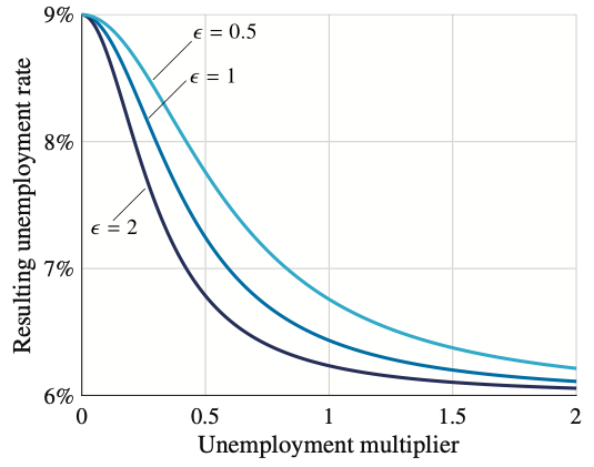
When the US government decided to implement the American Recovery and Reinvestment Act stimulus package in 2009, unemployment was projected to increase from 6% to 9% absent policy intervention. Given the properties of a well-designed stimulus package and the available empirical evidence, what should this stimulus package have looked like? The stimulus package resulting from our analysis is shown in Figure 1 for a realistic range of unemployment multipliers and elasticities of substitution between private and public consumption (The evidence on multipliers comes from Ramey 2013, and the evidence on the elasticity of substitution comes from Armano and Wirjanto 1998). As a complement, Figure 2 displays how much unemployment would have been reduced with the stimulus of Figure 1.
Figure 1 Optimal stimulus spending at the onset of the Great Recession in the US, given that unemployment was projected to increase from 6% to 9%
Notes: Stimulus spending is measured as a share of GDP. Each line represents the stimulus package for a range of possible values of the unemployment multiplier (percentage-point decrease in unemployment when public spending increases by 1% of GDP). The three lines differ by the value used for the elasticity of substitution between public and private consumption (ε).
Figure 2 Unemployment rate that would be reached with the stimulus package of Figure 1
Notes: We assume that the target efficient unemployment rate is 6% and that the economy has a 9% unemployment rate absent stimulus spending. Each line represents the unemployment rate that would be reached for a range of possible values of the unemployment multiplier (percentage-point decrease in unemployment when public spending increases by 1% of GDP). The three lines differ by the value used for the elasticity of substitution between public and private consumption (ε).
The stimulus package in Figure 1 illustrates the points that we have just discussed. First, even with a small multiplier (say 0.2), optimal stimulus spending is significant (above 1.5 percentage points of GDP). Second, the multiplier warranting the largest stimulus is fairly modest (between 0.3 and 0.6). Third, optimal stimulus spending is the same for small and large multipliers, and the resulting unemployment rates are of course very different. Fourth, for small multipliers, unemployment barely falls below 9%, although optimal stimulus spending is quite large. This is because public expenditure has little effect on unemployment when the multiplier is small. On the other hand, with a multiplier above one, stimulus spending almost brings back unemployment to its initial level of 6% (for instance, with a multiplier of one, the unemployment rate falls below 6.8%). Fifth, the higher the elasticity of substitution between public and private consumption, the higher the stimulus package. Yet, while the elasticity plays a significant role for small to medium multipliers, its role is much more limited for large multipliers. This is because for large multipliers, the optimal policy is essentially to fill the unemployment gap, so it is not influenced by the elasticity of substitution. Sixth, the stimulus package is plotted as a function of the unemployment multiplier, not the output multiplier, so all these results apply regardless of whether the taxes used to finance stimulus spending are distortionary or not.
References
Romer, C D and J Bernstein (2009), “The job impact of the American Recovery and Reinvestment Plan”.
Michaillat, P and E Saez (2019), “Optimal public expenditure with inefficient unemployment”, Review of Economic Studies 86(3): 1301-1331.
Ramey, V A (2013), “Government spending and private activity”, in Alesina, A and F Giavazzi (eds), Fiscal policy after the financial crisis, University of Chicago Press.
Amano, R A and T S Wirjanto (1997), “Intratemporal substitution and government spending”, Review of Economics and Statistics 79(4): 605-609.


