For years following the Great Financial Crisis, central banks struggled to get inflation back to their mandated targets. More recently, in the highly unusual post-Covid circumstances, inflation has risen considerably and has remained persistently above those targets, raising questions about its future evolution. One way to shed further light on these questions is to examine the inflation process at a very disaggregated level, i.e. by looking closely under inflation’s ‘hood’. Indeed, the recent run-up in inflation has involved outsize sector-specific price increases, caused in large part by supply bottlenecks that have had an uneven incidence across industries (Rees and Rungcharoenkitkul 2021).
In a recent paper, we explore the dynamics of inflation by considering the behaviour of 131 price indices of finely defined sectors in the US personal consumption expenditure (PCE) deflator over the period January 1959 to June 2020 (Borio et al. 2021).1 We reach two key findings, which, taken together, have significant implications for the conduct of monetary policy:
- First, once inflation settles at a low level, the contribution of the common component of price changes to inflation drops substantially and becomes relatively small. In other words, measured inflation is largely the result of idiosyncratic (relative) price changes. This is not what the theoretical definition of inflation is intended to capture, i.e. a generalised increase in prices.
- Second, in the low inflation environment that has prevailed since the early 1990s, changes in the monetary policy stance operate through a remarkably narrow set of prices, concentrated mainly in the more cyclically sensitive service sectors.
We next elaborate on the findings and their policy implications.
One index, two inflations…
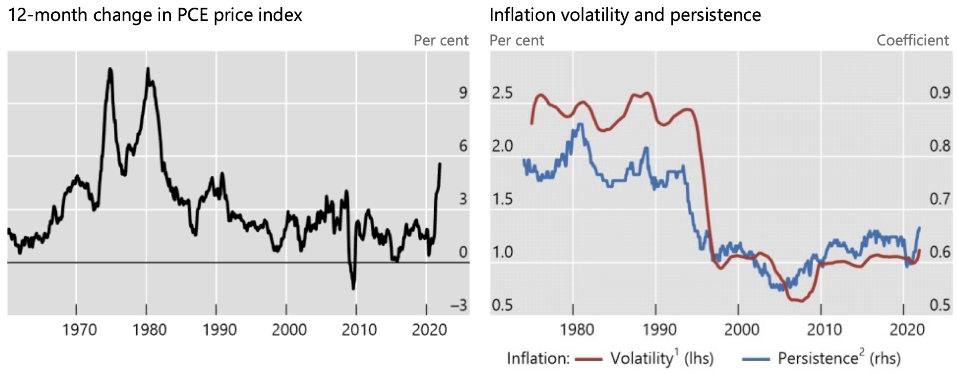
At the aggregate level, the properties of the inflation process are well known, as illustrated in the left-hand panel of Figure 1 in the case of the US. Inflation crept up in the late 1960s, surged in the 1970s and peaked at the turn of the 1980s, before dropping sharply in the wake of the so-called Volcker shock. Since the late 1980s, inflation has for the most part hovered within a narrow range until the recent pandemic-related disruptions. The volatility of inflation has tended to co-move with its level (the red line, right-hand panel). And so has the degree of persistence: once inflation has become lower, its changes have tended to die away more quickly (the blue line).2
Figure 1 US headline PCE inflation, its volatility and persistence
Notes: 115-year moving standard deviation of 12-month headline personal consumption expenditure (PCE) inflation. 2 A measure of persistence of one-month headline PCE inflation based on the estimator of mean reversion proposed by Dias and Marques (2010) and calculated using a 15-year rolling window.
Sources: US Bureau of Economic Analysis; author’s calculations.
Less well-known is that the inflation process has, if anything, changed even more at the disaggregated level. The left-hand panel of Figure 2 portrays an indicator of the co-movement of sector-specific prices, here simply captured by the time-varying share of the total variance of the 12-month percentage change in those prices explained by the first principal component estimated on a rolling 15-year window.3
Strikingly, the common component of price changes drops substantially alongside the inflation rate. For headline PCE inflation (the black line), it falls from over 50% to some 20% once the pre-1980 period of high and volatile inflation drops out of the estimation window. Similar patterns hold for the common components estimated for broad sectoral ‘inflation’ rates (services, durables and non-durables), as well as for narrower ones (not shown). And they hold equally for the transitory and trend components of inflation (also not shown).
A similar conclusion emerges by looking at the extent to which outsize (or “salient”) relative price increases pass through to core PCE inflation (centre panel). In other words, the so-called second-round effects, which would boost the importance of the common inflation component over time, appear to have become much smaller since the mid-1980s. We see that the distribution of pass-through estimates for the low inflation environment is much more concentrated around zero (compare the blue with the red line); in addition, the estimates are generally not statistically significant for this period.
Figure 2 The importance of the common factor underlying price changes has fallen sharply
Notes: 1 The common component of 12-month percent changes in prices across all sectors and within each specified broad PCE sector is estimated using a 15-year rolling window. 2 Each line shows the weighted kernel density estimate (ie a smoothed histogram) of the distribution of pass-through coefficients of “salient” relative price increases to 12-month ahead core personal consumption expenditure (PCE) inflation for the specified sample period. The weights are equal to the sector-specific average expenditure shares in each sample period. 3 Time-varying volatility of 12-month inflation is calculated using a 15-year rolling window. The calculation of variance and co-variance contributions to the total variance of 12-month headline PCE inflation is based on the 131 narrowly defined PCE sectors.
Sources: US Bureau of Economic Analysis; authors’ calculations.
Interestingly, the decline in the common component of inflation is the reason why the volatility of inflation has dropped so much. Most of the drop in the volatility does not reflect the decline in volatility within finely defined sectors, but rather the decline in the co-movement (covariance) of price changes across those sectors (right-hand panel). This pattern is analogous to the behaviour of the volatility of the yield on a portfolio of securities, where the co-movement of individual yields dwarfs the impact of the volatility of individual securities on the yield of the overall portfolio.
Monetary policy’s limited traction
Arguably, this evolution in the inflation process could, paradoxically, reduce the ability of changes in the monetary policy stance to influence inflation within a given policy regime. Intuitively, such changes should affect inflation primarily through aggregate demand and hence through the common component of price changes. All else equal, a smaller such component implies a smaller effect.
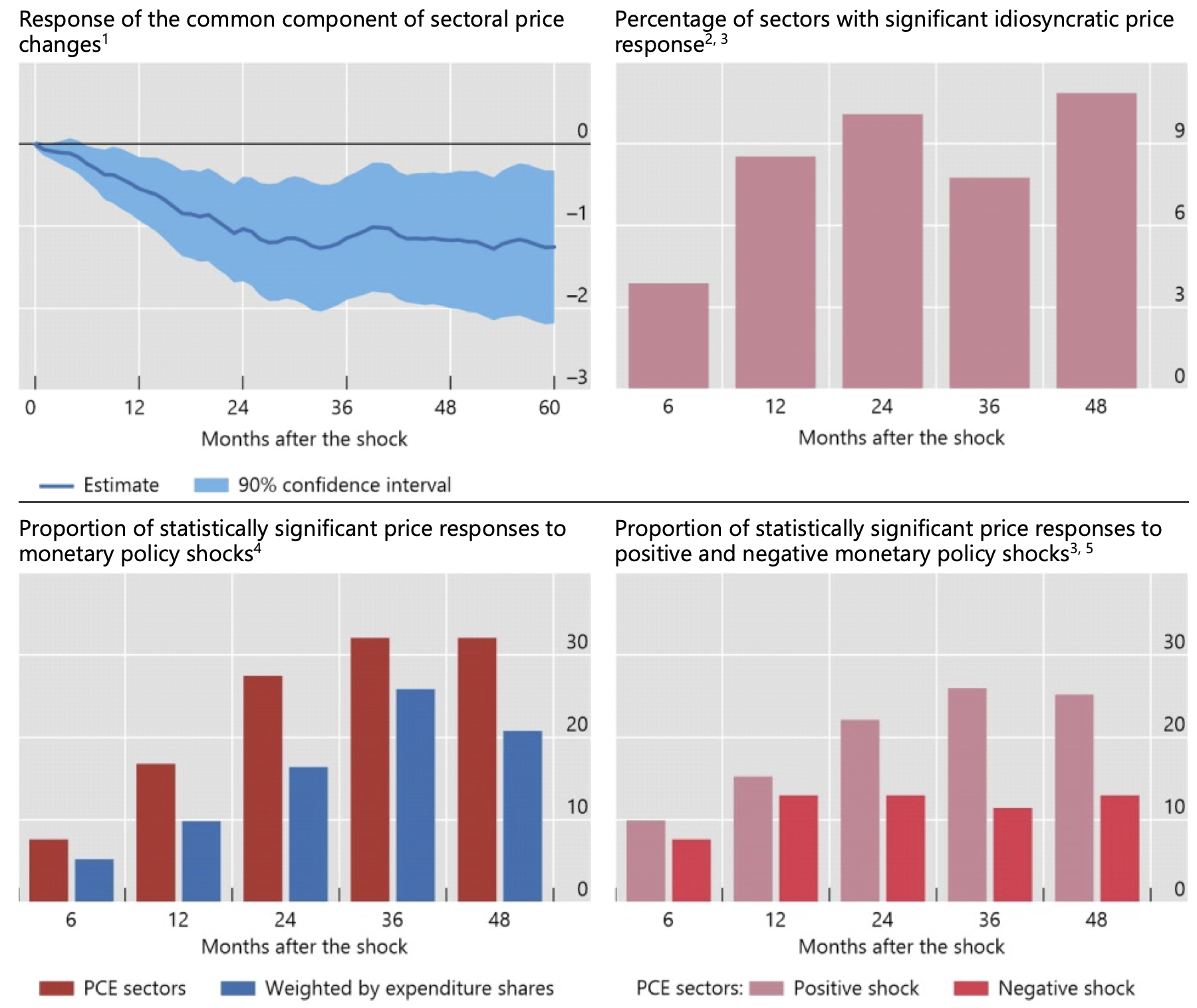
We find two pieces of evidence that are consistent with this hypothesis. We do so by examining the response of prices to carefully identified high-frequency monetary policy shocks, i.e. unanticipated changes in the stance of monetary policy, over the period July 1992–December 2018, controlling for a broad set of macroeconomic factors (Figure 3).
Figure 3 Monetary policy affects inflation primarily though the common component (%)
Notes: 1 The common component is constructed as the first principal component of monthly log price change across the 131 sectors. The solid line shows the accumulated response of the common component to a 25 basis points monetary policy shock in month 0. 2 For each sector, the idiosyncratic log price is calculated by summing up the residuals from the regression of monthly sector-specific log price changes on the common component. 3 Significant at 10% level. 4 Weighted percentiles of the response of prices across 131 narrowly defined personal consumption expenditure (PCE) sectors to a monetary policy shock of 25 basis points. The weights are equal to the sector-specific average expenditure shares. 5 In this specification, positive (ie contractionary) and negative (ie expansionary) monetary policy shocks of 25 basis points are allowed to have differential effects on sector-specific prices.
Sources: Board of Governors of the Federal Reserve System; US Bureau of Economic Analysis; Borio (2021); authors’ calculations.
First, as expected, changes in monetary policy operate largely through the common component of price changes: a contractionary monetary policy shock induces persistent disinflation over the medium term, as its impact on the common component of price changes is economically and statistically significant (top left-hand panel). The impact of the same shock on the various sector-specific price fluctuations, by contrast, is largely insignificant at conventional levels (top right-hand panel).
Second, over this period of low and stable inflation, changes in the policy stance appear to operate through a remarkably narrow set of prices. The impact on prices is statistically significant for only a small fraction of sectors – less than one fifth at the 10% significance level after 12 months (bottom left-hand panel). Even after 36 months, the fraction of sectors for which the price response is statistically significant rises to only about a third. Moreover, in terms of expenditure shares, the proportion is even lower across all horizons (same panel). The bulk of these sectors are in services, which on balance tend to be more sensitive to economic fluctuations.
Interestingly, not only is the response of prices to changes in the monetary policy stance relatively muted, but it also appears to be asymmetric. The fraction of sectors with statistically significant price responses is noticeably lower for expansionary than for contractionary monetary shocks, across all horizons (bottom right-hand panel). Ostensibly, monetary policy seems to be less effective in raising than in lowering inflation in such an environment.
Implications for monetary policy
What does this mean for the conduct of monetary policy in a low-inflation policy regime?
A key implication is the importance of flexibility. In other words, it may be neither feasible nor desirable to pursue tightly defined, precise inflation targets.5
It may not be feasible because the ability of monetary policy to steer inflation within narrow ranges is limited. Most of what we measure as inflation in such a low and stable inflation environment amounts, in effect, to relative price changes, over which adjustments in the policy stance have limited influence. And the set of prices over which those adjustments operate is remarkably small.
It may not be desirable because relative price changes tend not to feed much into generalised inflation: (i) because such adjustments are essential to a well-functioning economy – providing signals for appropriate resource reallocation – and, as such, should be accommodated, not resisted, by monetary policy;6 and (ii) because monetary policy’s limited leverage magnifies any collateral damage of sharp and prolonged shifts in the stance, not least the damage associated with interest rates that stay unusually low for unusually long (e.g. Borio 2020).
It is as if, after having worked hard to bring inflation down, the central bank can afford to enjoy the benefits. Just like a credible conductor of a well-rehearsed orchestra can afford to lead with minimal gestures, so a credible central bank can afford to let inflation evolve within a range of its target without energetic adjustments to the policy stance.
At the same time, the analysis also highlights the need for the central bank to remain alert. If measured inflation is allowed to rise back to higher, self-perpetuating levels, the environment becomes less welcoming. A stronger common component endangers the benefits of the central bank’s hard-earned credibility. It is one thing to tolerate significant, and possibly persistent, deviations from point targets; it is quite another to put the system’s self-equilibrating properties to the test.
Authors’ note: The views expressed are our own and do not necessarily reflect those of the Bank for International Settlements or the Bank of Thailand.
References
Adam, K and H Weber (2019), “Optimal trend inflation”, American Economic Review 103(2): 702–37.
Borio, C (2020), “When the unconventional becomes conventional”, remarks at “The ECB and Its Watchers XXI”, Frankfurt, 30 September.
Borio, C (2021), “Back to the future: intellectual challenges for monetary policy”, David Finch Lecture, University of Melbourne (also available as BIS Working Paper no 981).
Borio, C, P Disyatat, D Xia and E Zakrajšek (2021), “Inflation, relative prices and monetary policy: flexibility born out of success”, BIS Quarterly Review, September: 15–29.
Dias, D and C Marques (2010), “Using mean reversion as a measure of persistence”, Economic Modelling 27(1): 262–73.
Miranda-Agrippino, S and G Ricco (2021), “The transmission of monetary policy shocks”, American Economic Journal: Macroeconomics 13(3): 74–107.
Rees, D and P Rungcharoenkitkul (2021), “Bottlenecks: causes and macroeconomic implications”, BIS Bulletin 48.
Reis, R and M W Watson (2010), “Relative goods’ prices, pure inflation, and the Phillips correlation”, American Economic Journal Macroeconomics 2(3): 128–57.
Stock, J H and M W Watson (2002), “Macroeconomic forecasting using diffusion indexes”, Journal of Business and Economic Statistics 20(2): 147–62.
Wolman, A (2011), “The optimal rate of inflation with trending relative prices”, Journal of Money, Credit, and Banking 43(2–3): 355–84.
Endnotes
1 While we chose the US for our analysis because of the granularity and length of the available data, we expect the results to have more general validity, given the similarities in inflation processes across countries.
2 The convention here is that the data point labelled, say, “1990”, reflects an estimate based on the January 1975–December 1990 (15-year) window.
3 The first principal component is the linear combination of the underlying sectoral price changes that explains the highest fraction of the variance of overall inflation. It can be used as a proxy for the unobserved common component of all price changes. A dynamic factor model is another way to estimate the unobserved common inflation component (e.g. Reis and Watson 2010). Our more straightforward approach defines sector-specific price changes simply as idiosyncratic movements in sectoral prices that are unrelated to the common inflation component. Compared with dynamic factor models, our approach is easy to implement and computationally simple. As discussed in Stock and Watson (2002), the principal components consistently recover the space spanned by the factors when the cross-section is large, and the number of principal components used is at least as large as the true number of factors. Moreover, the principal component approach imposes fewer distributional assumptions on the data.
4 These high-frequency monetary policy shocks are constructed using the methodology developed by Miranda-Agrippino and Ricco (2021).
5 For an elaboration of this point in a broader context, see Borio (2021).
6 For an elaboration, see Adam and Weber (2019) and Wolman (2011).


