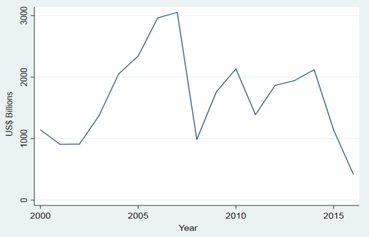
Was the 2015-16 sharp slowdown of capital flows, evident in both emerging market economies (EMEs) and advanced economies, part of a globalisation backlash? This question was in the minds of market participants and policymakers in late 2016. Globally, annual portfolio inflows fell well below the average of the preceding five years (Figure 1) and even below the amounts during the Global Crisis.
Figure 1 Global portfolio inflows to 2016
Was the slowdown in portfolio flows simply a temporary decline or did it represent something more long-lasting? How does one judge, in real time, if a slowdown in flows is abnormal (and thus likely to be temporary)? Bussière et al. (2016: 16) concluded that:
“it is hard to gauge if the pre-crisis properties and specificities of the various types of flows…will prevail in the ‘new normal’…. The changes that have taken place since the global financial crisis may correspond to a simple normalization, as suggested…by Coeuré (2015), after rather ‘exuberant’ times in the pre-crisis period.”
Creating a benchmark for portfolio flows
To gauge in real time if flows are abnormally high or low requires a benchmark. Exchange rates have a benchmark, purchasing power parity, that captures an intuitive long-term arbitrage in product markets and enables a narrative based on a potential mechanism of adjustment, rather than just an empirical trend. Economic activity (potential GDP), unemployment (natural rate or NAIRU), and interest rates (the natural rate of interest, r*) all have benchmarks. What is an appropriate benchmark for capital flows? Is there such a thing as a natural rate of capital flows?
In a recent paper, we create a benchmark for portfolio flows (Burger et al. 2018). Our benchmark is intuitive – it is the amount of new money available for international capital flows (that is, rest-of-the-world savings) allocated according to past portfolio weights. The benchmark is theoretically motivated by the Tille and van Wincoop (2010) notion of portfolio growth flows in which new savings are invested at steady state portfolio shares. Data requirements are not onerous – to construct the benchmark we only need data on savings (calculated using country level savings rates and GDP from the IMF’s World Economic Outlook) and portfolio weights (calculated based on data from Lane and Milesi-Ferretti 2018 on cross-border portfolio liabilities scaled by McKinsey Global Institute’s estimate of total financial assets). Our benchmark flows, which arise from rest-of-the-world macroeconomic conditions, represent the flows that recipient countries should expect regardless of what occurs in the local economy.
Empirical performance of the benchmark
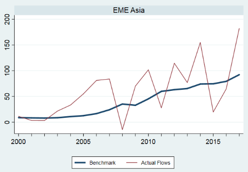
Figure 2 displays actual portfolio inflows with our natural rate for EME Asia and Latin America. Benchmark flows should not be mistaken as trend lines; they are derived from investor countries’ macroeconomic conditions (specifically rest-of-world GDP and savings rates). They do appear to be a ‘natural line' or long-run anchor around which actual flows oscillate. And what is apparent in Figure 2 is further supported by our empirical analysis: country-level error correction models provide evidence of a long-run cointegrating relationship such that inflows – especially EME portfolio inflows – adjust rapidly to the benchmark.
Figure 2 Benchmark and actual portfolio inflows for EME Asia and Latin America (annual, in billions of US$)
Having a benchmark provides context when investigating sharp movements in capital flows. For example, EME Asia’s portfolio inflows plummeted from US$155 billion in 2014 to US$20 billion in 2015 (Figure 2). Was the sharp decline in inflows surprising? Without a benchmark, one can only state (and analyse) the extent of the slowdown compared with some previous period. But Figure 2 reveals that the slowdown pushed EME Asia’s portfolio inflows below our benchmark, suggesting that the 2015 slowdown would likely be reversed (which indeed occurred in 2016/17). In contrast, the sharp 2015 decline in Latin America’s portfolio inflows was a return to benchmark levels, so our analysis suggests that 2016 and 2017 flows should be similar to those in 2015 (and indeed they were).
The recent dynamics of portfolio inflows into Latin America and EME Asia highlight an important feature of our analysis. Having a benchmark enables the differentiation of sharp movements away frombenchmark levels from sharp movements towardthe benchmark. Movements away from the benchmark are likely temporary, whereas movements toward the benchmark are likely to be sustained.
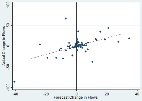
The statistically and economically significant tendency of actual flows to revert to the natural rate suggests observed deviations from the benchmark could be used to forecast future changes in portfolio flows. We test the out-of-sample forecasting ability of the benchmark by estimating an error correction model using 2000-2014 data and then forecasting the change in portfolio flows for 2015, 2016, and 2017. Figure 3 shows a scatterplot of the actual versus predicted change in portfolio flows for EMEs during the years 2015, 2016 and 2017 (i.e. three years for 28 EMEs, or 84 observations in all). It reveals an impressive performance of the error correction forecasting model; the correlation between actual and forecasted change in flows is 0.56 and most (57 of 84) observations lie in the first and third quadrants (in which the forecasted and actual changes have the same sign).
Figure 3 Model-based forecasts of changes in EME portfolio inflows
In many cases directional forecasts– forecasts of the direction of a change in an economic variable – can add considerable value, regardless of the statistical precision of the forecast. For example, policymakers and market participants might value the ability to forecast whether portfolio flows received by a particular country are likely to increase or decrease from current levels. We construct a simple benchmark-based forecast of the direction of the change in portfolio flows by assuming that flows will adjust toward the benchmark and find that for 65% of the 474 EME observations, the benchmark correctly forecasts the direction of the change in portfolio inflows.1
The empirical performance of our benchmark suggests there is a natural rate of portfolio inflows, a longer-term baseline path around which actual flows fluctuate (especially for EMEs), allowing observers to distinguish between movements toward the benchmark and movements away from the benchmark.
References
Burger, J D, F E Warnock and V C Warnock (2018), Benchmarking Portfolio Flows”, IMF Economic Review, forthcoming.
Bussière, M, J Schmidt and N Valla (2016), “International financial flows in the new normal: Key patterns (and why we should care)”, CEPII Policy Brief No. 10.
Coeuré, B (2015), “Paradigm lost: Rethinking international adjustments”, Egon and Joan von Kashnitz Lecture, Clausen Center for International Business and Policy, Berkeley, 21 November.
Lane, P, and G-M Milesi-Ferretti (2018), “The External Wealth of Nations Revisited: International Financial Integration in the Aftermath of the Global Financial Crisis”, IMF Economic Review 66(1): 189–222.
Pesaran, M H and A Timmermann (1992), “A simple nonparametric test of predictive performance”, Journal of Business & Economic Statistics 10(4): 461-465.
Tille, C and E van Wincoop (2010), "International Capital Flows", Journal of International Economics 80(2): 157-175.
Endnotes
[1] This performance is statistically significant, as the Pesaran and Timmermann (1992) test statistic of 6.57 strongly rejects the null hypothesis of predictive failure.


