With the spectre of a recession looming in the euro area, and elsewhere, the policy question that arises is how much leeway the fiscal authorities in the euro area have to follow counter-cyclical fiscal policies aimed at providing some stimulus. This question is important because it appears that the ECB’s capacity to provide for such a stimulus is limited. The ECB has flooded the markets with liquidity to the tune of trillions of euros since 2015. It is difficult to see how adding a couple of hundred billion of money base, most of which is likely to be hoarded or put to use for speculative activities, will provide for a significant stimulus of economic activity in the euro area.
The conclusion must be that the burden of business cycle stabilisation in the euro area will have to come from the fiscal authorities. This was also recognised by Mario Draghi when he announced a new dose of quantitative easing for the euro area (Hüther and Südekum 2019.).
Two questions arise about the use of fiscal policies. The first one is how effective these policies are in stimulating the economy. This is the question of the size of the fiscal multipliers. The second one is how much leeway the fiscal authorities have to perform their stabilisation responsibilities, taking into account that these authorities have significant levels of outstanding debt. There is considerable reluctance among policymakers these days to use fiscal policies for stabilisation purposes. This reluctance is mainly driven by the fear that these policies may lead to a surge in government debt and in so doing quickly become unsustainable.
Fiscal multipliers
There is a huge and longstanding literature on the size of the fiscal multiplier. Our contribution here is to present the results obtained in a behavioural macroeconomic model as developed in De Grauwe (2012), De Grauwe et al. (2019), and De Grauwe and Ji (2019).
In contrast with the existing rational expectations dynamic stochastic general equilibrium (DSGE) models, our model takes the view that agents have cognitive limitations preventing them from having rational expectations. Instead, these agents use simple rules of behaviour, i.e. heuristics. The model introduces rationality by assuming that individuals learn from their mistakes and are willing to switch to the better-performing rule. This model produces endogenous business cycles driven by ‘animal spirits’, i.e. market sentiments of optimism and pessimism that in a self-fulfilling way create booms and busts and are in turn influenced by these market movements. Our model seems to be appropriate to analyse the effectiveness of fiscal policies.
One important characteristic of this model is that the effects of policy shocks depend on the initial conditions, i.e. the state of the economy. This also means that the fiscal multipliers obtained in this model depend on the state of the economy. This is a key feature allowing us to analyse how fiscal policy can be used in different business cycle conditions.
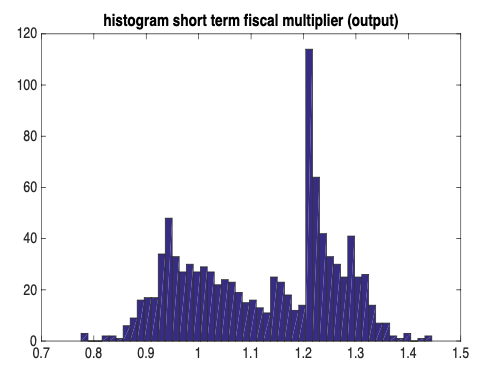
Figure 1 shows the results of computing the fiscal multipliers in the behavioural model under different initial conditions. We simulated 1,000 impulse responses of a positive government spending shock assuming each time different initial market sentiments, or animal spirits. Panel A shows the frequency distribution of the short-term fiscal multipliers, i.e. the response of GDP after four quarters. We observe a wide variation of these multipliers, from 0.8 to 1.5. We also note two peaks in the distribution: one around a multiplier of 1, and another around a multiplier between 1.2 and 1.3.
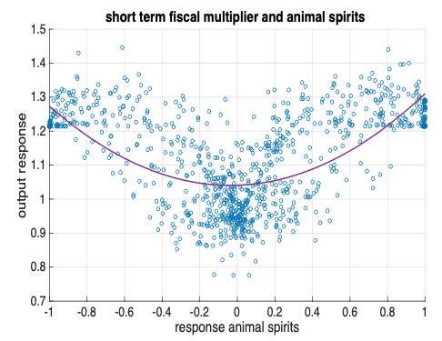
Panel B shows the origin of these two peaks. In the panel, we set out the fiscal multipliers on the vertical axis against the state of animal spirits in the initial period. These animal spirits are expressed as an index varying between -1 and +1. When the index equals -1 all agents are pessimistic, i.e. they forecast a decline in the output gap. When the index is +1, all agents are optimistic and forecast an increase in the output gap. When the index is 0, optimistic and pessimistic forecasts cancel out and the animal spirits are neutral. We find that when animal spirits are neutral (tranquil periods), the fiscal multipliers cluster around 1. When animal spirits take on extreme values, these fiscal multipliers cluster around 1.2 to 1.3. Thus, extreme values of animal spirits tend to amplify the effects of a fiscal expansion and lead to multipliers exceeding 1. Note, however, that there is still a lot of noise around the non-linear relation between fiscal multipliers and animal spirits, suggesting that other initial conditions affect the size of these multipliers.
There is increasing empirical support for the view that the size of the fiscal multipliers depends on the state of the economy. In a series of influential papers, Auerbach and Gorodnichenko (2012 and 2013) find that the size of fiscal multiplier is state-dependent in the US economy during the post-war period. In particular, they find that the multiplier exceeds 1 during recessions (see also Blanchard and Leigh 2013).
Figure 1 Short-term fiscal multipliers and animal spirits
Panel A
Panel B
Source: De Grauwe and Ji (2019)
Interest rate regimes and sustainability of fiscal policies
As mentioned earlier, there is considerable reluctance among policymakers to use fiscal policies for stabilisation because of a fear that these policies may lead to a surge in government debt and, in so doing, quickly become unsustainable. There is therefore a need to focus on issues of sustainability.
Sustainability is very much influenced by the interest rate regime countries face. It is well-known that when the nominal interest rate on public debt exceeds the nominal growth rate of GDP, the debt-to-GDP ratio will become unstable (will grow to infinity) unless the government produces a surplus on its primary budget balance, i.e. the budget balance that excludes interest payments.
Countries that experience an interest rate regime in which r > g, where r is the interest rate and g the growth rate of GDP, are therefore very much constrained in the use of fiscal policies. This is much less so in countries where r < g. In the latter countries, the inherent dynamics of the debt-to-GDP ratio will tend to be stable, i.e. even if the government finances all interest spending by debt issue, the debt-to-GDP ratio will tend to decline. There is therefore no need to produce a surplus in the primary budget balance. It is clear that, in the countries facing a favourable interest rate regime, there is no necessity for the fiscal authorities to finance interest spending by taxation. This has the effect of producing a softer budget constraint allowing for more choices in the use of fiscal policies for stabilisation purposes (see also Blanchard 2019.).
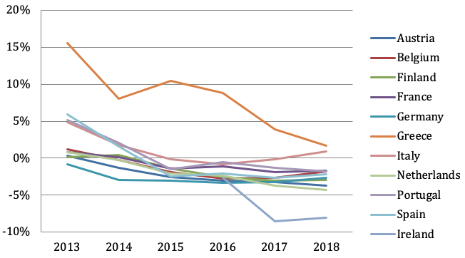
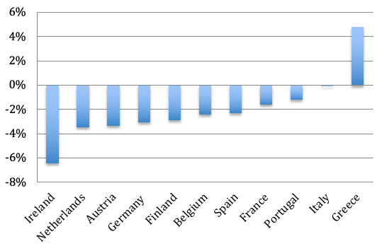
What is the interest rate regime prevailing in different euro area countries today? Figure 2 shows the evolution of r – g since 2013, the first year after the sovereign debt crisis. We observe that r – g declined in all euro area countries. The effect of this decline is that, with the exception of Greece and Italy, all euro area countries now profit from a favourable interest rate regime in which r-g < 0. In Figure 3, we take the average over the last three years and we come to the same conclusion, i.e. most countries of the euro area (except Greece and Italy) have been in a favourable interest rate regime.
Figures 2 and 3 use the market rates. This measures the marginal cost of issuing debt. The latter may diverge from the average interest cost of the government debt. Using the average interest cost instead of the marginal cost leads to similar results.
Figure 2 r - g in euro area countries (post-sovereign debt crisis)
Source: European Commission, AMECO
Note: Ireland was eliminated in 2015. This was the year Ireland had a growth rate of GDP exceeding 30%, resulting from special accounting procedures.
Figure 3 r - g (mean over 2016-18)
Source: European Commission, AMECO
Policy choices
Fiscal policies can be used to stabilise output. The sustainability depends on the interest rate regime and therefore determines the choices faced by the fiscal authorities. We analyse these choices using again our behavioural macroeconomic model.
We did this by computing the trade-offs the fiscal authorities face between stabilising output and debt in our behavioural model, assuming that the debt is kept sustainable. As indicated earlier, this model takes into account the state of the economy when the authorities engage in counter-cyclical fiscal policies.
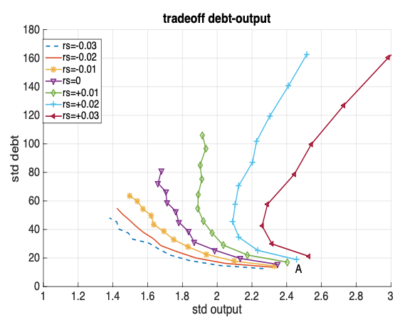
We show the trade-offs between volatility of output and public debt in Figure 4. In order to understand this trade-off it is good to start from point A. This shows the points of the trade-offs when there is no fiscal stabilisation, i.e. the fiscal authorities do not follow counter-cyclical policies. As they increase their counter-cyclical fiscal policies, we move up along the trade-offs.
We distinguish between different interest rate regimes, called rs, where rs = r – g. We allow rs to vary from -3% to + 3%. Let us first concentrate on rs = r – g < 0. In this regime, we obtain negatively sloped trade-offs, i.e. when fiscal authorities increase their output stabilisation efforts this comes at a price of increasing the variability of the debt. When rs = -0.03, this negative trade-off is relatively flat, i.e. the cost of output stabilisation in terms of debt variability is small. With increasing rs, the slope of the trade-offs increases, which indicates that the cost of stabilisation tends to increase.
When rs = r – g turns positive, we observe that these trade-offs tend to bend backwards. Thus, in this interest rate regime when anti-cyclical fiscal policies become strong enough, the trade-offs become positively sloped, i.e. further attempts at stabilising output by varying government spending lead to increases in both the variability of output and debt. Further attempts to use counter-cyclical fiscal policies then reduce welfare. What is the intuition behind this result?
In order to understand this result, let us analyse what happens during a recession. If the fiscal authorities increase spending in order to stabilise output, this leads to increases in the deficit and thus in government debt. We know, however, that when rs > 0 the debt is dynamically unstable except if the authorities keep a sufficiently positive primary balance. The counter-cyclical fiscal policy, however, leads to a departure from this condition, thereby destabilising the debt. The latter forces the fiscal authorities to reduce spending, thereby offsetting the counter-cyclical policy stance. When rs is very positive, the underlying instability of the debt is very strong. As a result, the need to reduce spending to stabilise the debt overwhelms the counter-cyclical policy stance. Fiscal policies as a whole become pro-cyclical. Attempts to stabilise output lead to more variability of output and debt.
From the preceding, it follows that, in interest rate regimes in which the interest rate exceeds the growth rate of the economy, the use of fiscal policy to stabilise output is severely limited. The use of fiscal policy to stabilise the business cycle can quickly lead to a loss-loss situation in which both the government debt and the business cycle are destabilised. In a regime where the interest rate is lower than the growth rate of the economy, this problem does not arise. This is a regime that allows the fiscal authorities to follow counter-cyclical policies without destabilising government debt.
Where should one locate the different euro area countries in this analysis? We have seen that countries like Austria, Ireland, the Netherlands, Germany, Belgium, Spain and Finland are in an interest rate regime where r – g is close to -2% or lower. France and Portugal are also in a favourable interest rate regime, but less spectacularly so. This means that these countries face favourable trade-offs, which allows them to use anti-cyclical fiscal policies without destabilising their government debts. Italy and Greece, however, do not face these favourable trade-offs and risk destabilising their government debt if they were to engage in intense anti-cyclical policies.
Figure 4 Trade-off between variability of output and debt
We conclude that, on the whole, most euro area countries today have the capacity to use fiscal policies as a tool to fight a looming recession without the risk of destabilising their government debt levels.
Conclusion: Changing budgetary priorities in the euro area
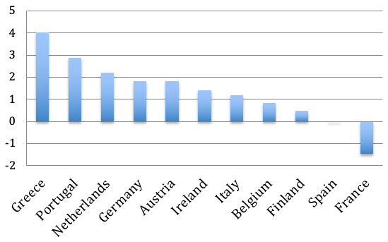
The previous conclusion can be strengthened by analysing the primary budget balances of the euro area countries shown in Figure 5 and comparing these with the interest rate regimes shown in Figure 2. The most striking aspect of this comparison is that most euro area countries show primary surpluses while they are in a favourable interest rate regime, i.e. r – g < 0. The latter would allow them to run primary deficits while keeping their debt-to-GDP ratios constant. This reflects a policy choice in most euro area countries that prioritises a speedy decline in debt-to-GDP ratios. The issue is whether this policy choice continues to make sense when the euro area economy is slowing down.
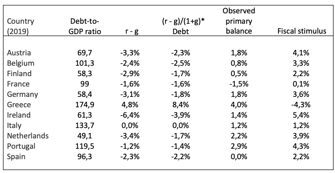
In Table 1, we compute the primary balances that are needed for the debt-to-GDP ratios to remain constant in the euro area countries (see the column labelled “(r-g)*Debt”). We compare these with the observed primary balances. The difference between the two tells us how much fiscal stimulus these countries could engage in while keeping their debt-to-GDP ratio at the levels reached in 2019. The results of this calculation are presented in the last columns. These results are striking. Most euro area countries are in a situation in which they could engage in a fiscal stimulus of more than 2% of their GDP, with some countries reaching 3% or more, while keeping their debt-to-GDP ratios fixed. The exceptions are Greece, Italy and France, which have no leeway for stimulus (Greece) or relatively little (Italy and France).
One note of warning is in place here. The numbers in the column (r-g)/(1+g)*Debt identify the necessary condition for debt sustainability. They may not be sufficient. Take Portugal for example. The number -1.4% says that Portugal could have a primary deficit of 1.4% that will keep the existing debt-to-GDP ratio constant at the level of 119.5%. That level, however, could be considered unsustainable in the face of some unfavourable shocks. Portugal, therefore, may not want to use fiscal stimulus today.
Figure 5 Primary budget balances as a % of GDP, 2019
Source: European Commission, AMECO
We conclude that a significant number of euro area countries (Austria, Germany, Ireland, Netherlands and Finland) could engage in a fiscal stimulus of 3% or more of their GDP. The choice these countries face today is the following. They can either go on the path of sharp declines of their debt-to-GDP ratios, even in the face of a recession. Or they can judge that, with the present threat of a recession, a (temporary) stop in the decline in their debt ratios is desirable. Such a decision would create a fiscal space allowing them to stimulate their economies by 3% to 4% of GDP, a stimulus that would surely do much in preventing a serious recession. Thus, these countries should consider changing their budgetary priorities skewed towards fast reductions of their debt-to-GDP ratios towards one prioritising a fiscal stimulus.
Table 1
Note: the column (r-g)/(1+g)*Debt measures the primary balance that will keep the debt-to-GDP ratio at the level of 2019; the last column measures the size of the fiscal stimulus in each country that will keep the debt-to-GDP ratio fixed at the level of 2019, given (r – g) in 2019.
References
Auerbach, A and Y Gorodnichenko (2012), “Measuring the output responses to fiscal policy”, American Economic Journal: Economic Policy 4(2): 1–27.
Auerbach, A and Y Gorodnichenko (2013), “Fiscal multipliers in recession and expansion”, in A Alesina and F Giavazzi (Eds), Fiscal Policy after the Financial Crisis, 63–98, Chicago: University of Chicago Press.
Blanchard, O and D Leigh (2013), "Growth forecast errors and fiscal multipliers", IMF Working Papers, No. 13/1, Washington, D.C.
Blanchard, O (2019), "Public debt and low interest rates", AEA Presidential Lecture, January,
De Grauwe, P (2012), Lectures on behavioral macroeconomics, Princeton University Press.
De Grauwe, P, P Foresti and Y Ji (2019), "Fiscal policies in booms and busts", CEPR Discussion Paper No. 13740.
De Grauwe, P and Y Ji (forthcoming), Behavioral macroeconomics. Theory and Policy, Oxford University Press.
Hüther, M and J Südekum, J (2019), "The German debt brake needs a reform", VoxEU.org, 6 May.
