The unexplained part of public debt

The answer to the question “How do countries get into debt?” seems trivial. The stock of debt is equal to the sum of past budget deficits. Countries accumulate debt whenever they run a budget deficit and reduce their debt when they run a budget surplus. In fact, the standard Economics 101 textbook debt accumulation equation states that the change in the stock of debt is equal to the budget deficit (for those who like equations this can be expressed as:  DEBTt – DEBTt-1 = DEFICITt ).

However, anyone who has worked with actual debt and deficit data knows that debt accumulation can be better described as the sum of deficit plus an unexplained residual. Formally, this can be written as: DEBTt – DEBTt-1 = DEFICITt + SFt ,where SFt measures the stock-flow reconciliation, a cumbersome name that comes from the fact this residual entity reconciles the deficit, which is a variable measured over a period of time (ie, a ‘flow’ variable), with debt, which is a variable measured at a given moment (ie, a ‘stock’ variable). We like to call this term ‘the unexplained part of public debt’.

The textbook equation is a good approximation for debt accumulation if we assume that the unexplained part of debt is not very large. But is this the case? Let us consider a couple of examples (the list could be much longer). In December 1998, Brazil’s net public debt stood at approximately 42% of GDP, but by January 1999 Brazil’s public debt surpassed 51% of GDP. Could the Brazilian government have run a fiscal deficit of almost 10% of GDP in just one month? Uruguay presents another interesting case. In March 2002, Uruguay’s debt was 55% of GDP, yet by the end of 2003 debt had soared to 110% of GDP. Could the Uruguayan authorities have run a deficit of 55% of GDP in less than two years? Finally, let's look at Argentina. In 2001 Argentina’s debt was just above 50% of GDP. By 2002 Argentina's debt was well above 130% of GDP. Did Argentina really run a deficit of 80% of GDP in just one year? IDB (2006) describes how these sudden debt explosions relate to the unexplained part of public debt. It is worth noting that the unexplained part of debt is not only an emerging market phenomenon. In a recent Vox piece, Cafiso (2012) shows that the unexplained part accounts for nearly one third of public debt growth in EU15 countries over 2008–10.

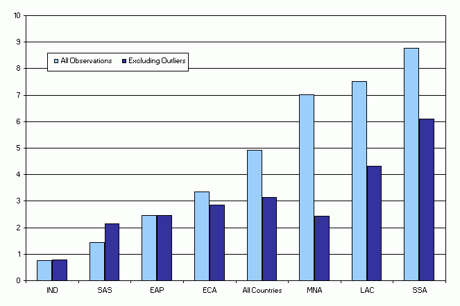
In Campos et al (2006), we move beyond anecdotal evidence and use data for 117 countries over a period of 30 years (1972–2003) to show that in the average country-year, debt grows 3 percentage points of GDP faster than what is implied by the budget deficit (this value is obtained after dropping outliers; if outliers are included in the sample, the average unexplained change in debt reaches 5% of GDP,  as in Figure 1). The highest values are in sub-Saharan Africa, Latin America and the Caribbean, and the Middle East. While debt and deficit data tend to be noisy, random measurement error would have yielded a zero average.

Figure 1. The Unexplained part of public debt (percent of GDP)

Note: IND: Advanced economies; SAS: South Asia; EAP:East Asia and Pacific; ECA: East Europe and Central Asia; MNA: Middle East and North Africa; LAC: Latin America and Caribbean; SSA: sub-Saharan Africa

Source: Campos et al (2006) and IDB (2006)

Another way to assess the importance of the stock-flow reconciliation is to divide both sides of the equation discussed above by GDP and use it to estimate the following statistical model:

                                        

where dt,i is the change in debt divided by GDP, deft,i is deficit over GDP, αi is a country-specific parameter (this parameter controls for the fact that the data come from different sources, countries have different levels of debt, and they use different methodologies for computing debt and deficit), and εt,i is the error term of this statistical model. The R2 statistics measure the goodness of fit of this model by calculating the share of variance of the dependent variable (dt,i) which is ‘explained’ by the independent variables (in this case deft,i). If the unexplained part of debt growth were unimportant, the above equation should fit the data well and yield an R2 close to one. An R2 of zero would instead indicate that there is no relationship between the dependent and the explanatory variables.

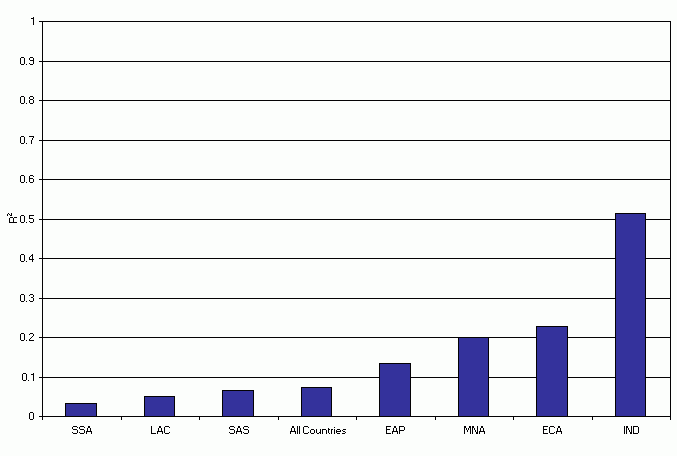
Figure 2 describes the R2s obtained by estimating the equation described above for different subsamples of countries. It shows that when all countries are pooled together, the R2 is just above 0.07, indicating that deficits explain 7% of the change in debt (and the stock-flow reconciliation 93%) – a very poor explanatory power for an equation which is often considered to be an identity. Even in the advanced economies, recorded budget deficits only explain 50% of debt growth.

Figure 2. Debt and deficit: Goodness of fit

Note: ECA: Eastern Europe and Central Asia, EAP: East Asia, IND: Industrial Countries, LAC: Latin America and Caribe, SAS: South Asia, MNA: Middle East and North Africa, SSA: Sub-Saharan Africa.

So far, we looked at the change in debt divided by GDP. However, for good reasons, policy discussion and fiscal sustainability assessments tend to focus on the evolution of the debt-to-GDP ratio. The growth rate of the debt-to-GDP ratio can be divided into five components: inflation, real GDP growth, interest expenditure, primary deficit (interest expenditure and primary deficit add up to the total deficit), and the unexplained part.

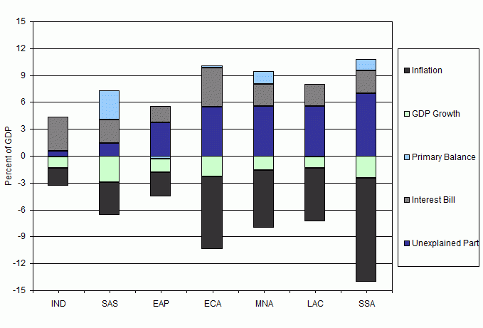
By applying this decomposition to a large number of countries over the period 1972–2003, we find that inflation and GDP growth are the main drivers of debt reduction (Figure 3). Curiously, the effect of inflation dominates that of real GDP growth in every region of the world (this is partly due to financial repression; see Reinhart and Sbrancia 2011). In the advanced economies and South Asia budget deficits are the main determinants of debt accumulation. In all other regions of the world, the unexplained part of public debt is the key determinant of debt accumulation.

Figure 3. Decomposition of debt growth in different regions of the world  (average 1972–2003)

Note: ECA: Eastern Europe and Central Asia, EAP: East Asia, IND: Industrial Countries, LAC: Latin America and Caribe, SAS: South Asia, MNA: Middle East and North Africa, SSA: Sub-Saharan Africa.

Source: Campos, Jaimovich, and Panizza (2006) and IDB (2006)

After having documented that there are large differences between deficits and changes in debt, we can explore the determinants of these differences. In Campos et al (2006), we use a statistical model that tries to explain the unexplained part of debt with three types of variables. We first look at the interaction between currency depreciations and the presence of foreign currency debt and find that depreciations lead to large stock-flow reconciliations in countries with high levels of foreign currency debt. Next, we look at the resolution of sovereign default episodes (for a survey of the recent literature on sovereign debt and default, see Panizza et al 2009) and, as expected, we find that defaults are associated with a negative unexplained part of debt (approximately 2% of GDP). Finally, we consider the role of banking crises. These are important events that generate contingent liabilities and other unrecorded off–balance sheet activities that can translate into debt explosions. We find that the average banking crisis is associated with a stock-flow reconciliation of almost 3% of GDP.

While these results suggest that building a safer debt structure and implementing policies aimed at limiting the creation of contingent liabilities are key to avoiding debt explosions, we also note that the above variables only explain 20% of the variance of the stock-flow reconciliation. There are two possible reasons why the statistical model described above does such a poor job at uncovering the determinants of the unexplained part of debt.

The first has to do with the fact that measurement errors that lead to an underestimation of the deficit are more important in some countries than in others. This is consistent with the findings of Aizenman and Powell (1998), who suggest that governments have incentives to misreport public expenditure and that this comes back to haunt them as debt is re-assessed in the future.

The second is that the importance of contingent liabilities that lead to debt explosions varies across countries and that the control variables included in the statistical exercise described above do not capture all the possible sources of contingent liabilities.

The fact remains, however, that irresponsible fiscal policy is not always the culprit of debt explosions.

Editor's Note: This article draws on Chapter 3 of IDB (2006) and on Campos et al (2006).

References

Aizenman, Joshua and Andrew Powell (1998), "The political economy of public savings and the role of capital mobility", Journal of Development Economics, 57(1):67-95.

Cafiso, Gianluca (2012), "Understanding Eurozone debt developments by nation", VoxEU.org, 5 January.

Campos, Camila, Dany Jaimovich, and Ugo Panizza (2006), "The unexplained part of public debt", Emerging Markets Review, 7(3):228-243.

Inter-American Development Bank (2006), Living with Debt, Harvard University Press.

Panizza, Ugo, Federico Sturzenegger, and Jeromin Zettelmeyer (2009), "The Economics and Law of Sovereign Debt and Default", Journal of Economic Literature, 47(3):651-698.

Reinhart, Carmen, and M Belen Sbrancia (2011), “The Liquidation of Government Debt”, NBER Working Paper No. 16893.