An economy’s income reflects payments to labour, rental payments to capital, and economic profits that emerge when prices exceed average production costs. In practice, it is very difficult to differentiate between these three categories. Labour compensation reflects more than just wages, and it is difficult to measure the value of benefits, stock options, and other transfers of value to compensate for workers’ time. Capital rental payments are generally implicit rather than explicit because firms typically own rather than rent their factories, machines, and brands. For this reason, economists and statisticians typically impute payments to capital using a user cost formula as in Hall and Jorgenson (1967). Finally, economic profits are hard to measure since data on average costs are rare.
It is perhaps not surprising, therefore, that comparing US GDP to the sum of standard measures of payments to labour and imputations of payments to capital results in a large and volatile residual term that we term ‘factorless income’. In a new paper (Karabarbounis and Neiman 2018), we consider three strategies for interpreting and allocating factorless income. First, we treat it as if it entirely reflects economic profits or rents, what we call Case Π. Second, we construct a series for unmeasured investment flows such as intangibles that might result in variation in factorless income, what we call Case K. Finally, we study the possibility that typical implementations of the Hall-Jorgenson formula, at least for the purposes of measuring medium-frequency movements at the aggregate level, miss important elements driving production decisions including risk premia, financial conditions, and adjustment costs, our Case R. We are not the first to consider these three cases. Indeed, a large set of papers either implicitly or explicitly makes one of these three assumptions. Rather, our work offers a unified empirical exploration of all three cases, comparing and evaluating their implications for the paths of technology and drivers of the labour share, growth, and inequality. We offer evidence that Case Π is the least compelling, offer a methodology to explore Case K, and conclude that Case R is the most promising interpretation of factorless income.
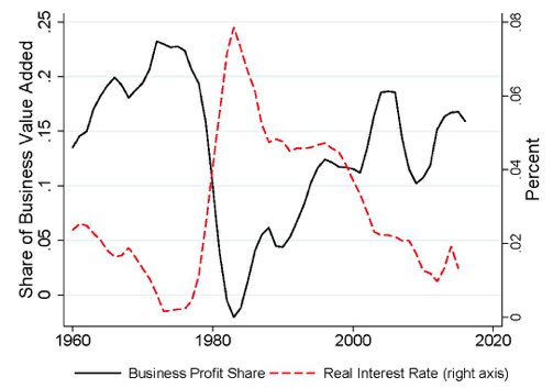
Figure 1 Profit share (i.e. ‘factorless income’) and the interest rate, US business sector
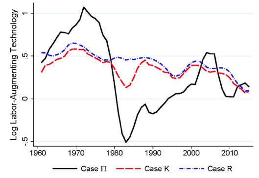
The black line in Figure 1 shows the path of factorless income under the interpretation of Case Π, so its share is simply relabelled as the profit share. Several papers, including Barkai (2016) and Eggertsson et al. (2018), implement the same or similar methodology and have focused on the increasing profit share since 1980 as the likely driver of the declining labour share during that same period, a global phenomenon uncovered in our own earlier work (Karabarbounis and Neiman 2014). Extending the calculation back in time, however, reveals that factorless income was high as a share of GDP in the 1960s and 1970s, before collapsing around 1980 and then slowly returning today to just below its levels earlier in the sample. If this methodology were to be used, therefore, to support, for instance, tighter antitrust enforcement, it should be acknowledged that similar logic would have applied for most decades in the post-war era.1 Further, a comparison with the real interest rate (plotted as the dashed red line in Figure 1) clarifies what, mechanically, underlies the inference in Case Π. Imputed capital costs move nearly one-to-one with movements in the interest rate and, therefore, drive the profit share’s behaviour.2 Finally, Figure 2 plots the detrended path of labour-augmenting technology for each of these three cases under a production function with an elasticity of substitution between capital and labour (σ) of 1.25.3 The variability of labour relative to capital costs under Case Π requires an unreasonably variable path of technology, as shown in the solid black line. For all these reasons, we are sceptical of this case and do not feel it is compelling enough to support new policies.
Figure 2 Implied labour-augmenting technology (detrended, σ= 1.25)
Case K reflects the view that some expenditures in the economy should best be thought of as investments, even though they may be captured by national statisticians as spending on intermediate inputs. For example, expenditures to train workers or build a firm’s brand equity look in income statements the same as purchases of raw materials, but they are done not as a requirement of production but rather to enhance the scale of future production.4 We develop a procedure to construct sequences for the price and quantity of unmeasured investment flows that would fully account for all changes in factorless income. Among these feasible sequences, we look for paths that seem plausible and offer one where the unmeasured spending typically averages only a few percentage points of GDP and the implied total factor productivity (TFP) series (the dashed red line in Figure 2) is dramatically more stable than that under Case Π. As discussed in our paper, however, our implementation of this case also carries with it the puzzling observation that the scale of the unmeasured capital stock is implausibly large at the beginning of our sample.
Finally, Case R explores the possibility that variation in factorless income is attributable to differences in the opportunity cost of capital internalised by firms when making production and investment decisions and standard measures of this cost such as those based on the yields of ten-year Treasuries. We solve for an alternative path for the opportunity cost faced by firms that would generate different rental rates that eliminate all variation in factorless income. This alternative series does not decline since 1980 as do Treasury rates, consistent with the view expressed by Caballero et al. (2017) that equity risk premia have increased over that period. Further, as shown in the blue dot-dashed line in Figure 2, this interpretation renders what we view as the most natural path for technology among the three cases. For these reasons, we view Case R as most promising for further exploration, though we acknowledge that full acceptance of this case demands direct evidence on the driver of the gap between firms’ cost of capital and Treasury rates (such as direct evidence on risk premia), including back to 1960 when the implied opportunity cost was at historic highs.
The interpretation and allocation of factorless income has critical implications for views on technology, product market competition, capital market frictions, inequality, and a host of other policy-relevant topics. We hope that our framework and methodology leads to rigorous examination of these three cases both in the US and around the world.
References
Barkai, S (2016), “Declining labor and capital shares”, University of Chicago working paper.
Caballero, R, E Farhi and P-O Gourinchas (2017), “Rents, technical change, and risk premia”, American Economic Review 107(5): 614-620.
Corrado, C, C Hulten and D Sichel (2009), “Intangible capital and US economic growth”, Review of Income and Wealth 55(3): 661-685.
Eggertsson, G, J Robbins and E Wold (2018), “Kaldor and Piketty’s facts: The rise of monopoly power in the United States”, NBER Working Paper 24287.
Eisfeldt, A and D Papanikolaou (2013), “Organization capital and the cross-section of expected returns”, Journal of Finance 68(4): 1365-1406.
Hall, R and D Jorgenson (1967), “Tax policy and investment behavior”, American Economic Review 57(3): 391-414.
Karabarbounis, L and B Neiman (2014), “The global decline of the labor share”, Quarterly Journal of Economics 129(1): 61-103.
Karabarbounis, L and B Neiman (2018), “Accounting for factorless income”, NBER Working Paper 24404.
McGrattan, E and E Prescott (2005), “Taxes, regulations, and the value of US and UK corporations”, Review of Economic Studies 72(3): 767-796.
Endnotes
[1] Further, the longer time series makes clear that this methodology for measuring economic profits is at odds with, rather than reinforcing of, the results in De Loecker and Eeckhout (2017), which are based on firm-level data and show that markups were largely flat prior to 1980 before rising to record levels today.
[2] Figures 1 and 2 here plot all series as five-year moving averages.
[3] The paper repeats all relevant plots with a lower elasticity of substitution (equal to 0.75). Our results, comparisons, and conclusions on the plausibility of the three cases do not qualitatively change.
[4] Influential work along these lines has been done by McGrattan and Prescott (2005), Corrado et al. (2009) and Eisfeldt and Papanikolaou (2013).


