In the past, US inflation used to rise during economic booms, as businesses charged higher prices to cope with increases in wages and other costs. When the economy cooled and joblessness rose, inflation declined. This pattern changed around 1990. Since then, US inflation has remained remarkably stable, even though economic activity and unemployment have continued to fluctuate. For example, shortly after the Great Recession, the unemployment rate reached 10%, but inflation barely dipped below 1%, leading many economists to look for the ‘missing deflation’ (e.g. Ball and Mazumder 2011). More recently, with unemployment below 5% for almost four years and inflation persistently under 2%, attention has turned to explaining what is holding inflation back (e.g. Powell 2019, Yellen 2019).
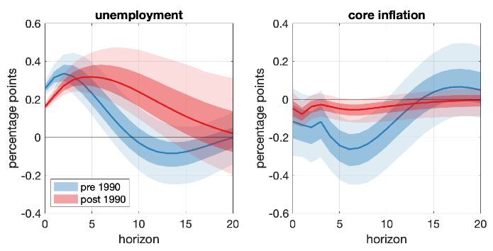
In a recent paper (Del Negro et al. 2020), we illustrate this phenomenon by plotting the dynamic responses of PCE inflation and the unemployment rate to a surprise increase in the latter, based on a vector autoregressive (VAR) model. As shown in Figure 1, when these responses are computed using data before 1990 (in blue), core inflation drops significantly. However, when they are computed using data after 1990 (in red), core inflation barely moves. The responses of unemployment, in contrast, are pretty similar across the two samples. Other economies, such as the euro area, have also experienced similar patterns (e.g. Constâncio 2015, Bobeica and Jarocinski 2017, Eser et al. 2020).
Figure 1 Responses of unemployment and core PCE inflation to an unemployment shock
Note: Impulse responses obtained using a VAR estimated with data before (blue) and after (red) 1990. The solid lines are posterior medians, while the shaded areas correspond to 68% and 95% posterior credible regions. Please see the paper for additional details.
Is the stability of US inflation due to changes in the functioning of labour markets, a flatter Phillips curve, or improved monetary policy?
What explains the emergence of this disconnect between inflation and unemployment? Economists have explored three main classes of explanations.
- The functioning of labour markets has changed in the last three decades, making unemployment a poorer indicator of both the degree of resource underutilisation in the economy (sometimes referred to as ‘economic slack’) and of the cost pressures faced by firms.
- Firms’ pricing decisions have become less sensitive to these cost pressures. In economic jargon, this phenomenon corresponds to a flattening of the Phillips curve – a relationship capturing the fact that a boost in production typically pushes up the cost of production inputs, and thus leads to higher output prices.
- Policy has become more successful in stabilising inflation (McLeay and Tenreyro 2019).
In Del Negro et al. (2020), we discuss the relative merit of these three explanations based on evidence from a combination of state-of-the-art macroeconometric techniques.1 The bulk of this empirical evidence points towards the second explanation – a flatter Phillips curve due to the reduced sensitivity of firms’ pricing decisions to their cost pressures – as the main driver of inflation stability. In terms of policy, this finding implies that inflation has become harder to steer, unless monetary authorities systematically take into account the flattening of the Phillips curve. Not surprisingly, the analysis of the ‘health’ of this relationship has taken centre stage in the strategic review recently undertaken by the Federal Reserve System, as highlighted by Chair Powell in his Jackson Hole speech, and currently under way at the ECB and other central banks.
Our findings
Figure 2 suggests that the first hypothesis is unlikely to be the main story. It shows the response of various measures of economic slack and cost pressures – such as GDP, hours worked, and unit labour costs – to the unemployment shock mentioned above. The responses of all these variables are very similar before and after 1990. This suggests that the stability of inflation over the past 30 years is not due to a break in the cyclical behaviour of any specific measure of slack or cost pressures. This observation arguably rules out changes in the functioning of labour markets as a leading explanation for the inflation-business cycle disconnect.
Figure 2 Responses of GDP, hours worked per capita, the labour share to an unemployment shock
Note: Impulse responses obtained using a VAR estimated with data before (blue) and after (red) 1990. The solid lines are posterior medians, while the shaded areas correspond to 68% and 95% posterior credible regions. Please see the paper for additional details.
This leaves us with two possible explanations on the table: a flatter Phillips curve and improved monetary policy. We discriminate between them by studying the effects of sudden changes in the economy-wide demand for goods and services – or, more precisely, unanticipated demand shocks. Monetary policy can limit their impact on inflation by ‘leaning against the wind’, that is, by counteracting their effects on economic activity as well. Therefore, if improved monetary policy is behind inflation stability, these demand shocks should have minor effects both on inflation and unemployment after 1990. In contrast, if inflation stability is due to limited sensitivity of prices to cost pressures and a flatter Phillips curve, demand shocks would continue to have a large impact on unemployment, although not on inflation.
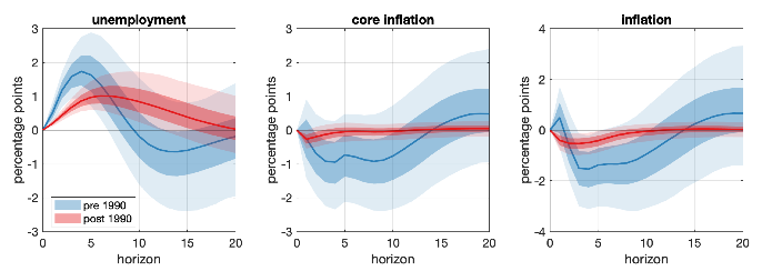
Figure 3 plots the responses of unemployment and inflation to a demand shock before and after 1990.2 The last two panels show that the response of inflation to demand shocks has indeed become significantly more muted since 1990. As for unemployment, its response appears to have been attenuated in the first few quarters but it has also become more persistent, leading to a larger cumulative effect over a five-year horizon.
Figure 3 Response of unemployment and inflation to a demand shock
Note: Impulse response of the unemployment rate, core PCE inflation and PCE inflation to a demand shock of the same size in the pre-1990 sample (blue) and post-1990 sample (red). The solid lines are posterior medians, while the shaded areas correspond to 68% and 95% posterior credible regions. Please see the paper for additional details.
These empirical results are consistent with the common narrative behind the Great Recession. Although its origins are complex, most observers agree that the recession was mostly associated with a collapse in demand due to the credit tightening brought about by the preceding financial crisis. If this analysis is correct, the fact that economic activity collapsed while inflation did not fall substantially suggests that the Phillips curve must be flat. This flattening of the Phillips curve is also what we find by estimating the New York Fed DSGE model before and after 1990.3
Investigating the deeper forces behind the flattening in the Phillips Curve is outside the scope of our analysis and it is still an open question in the specialised literature. The most prominent hypothesis attributes the reduced responsiveness of prices to cost pressures to the increased relevance of global supply chains, heightened international competition, and other effects of globalisation (e.g. Sbordone 2007, Forbes 2019). Understanding this further is of first-order importance for central banks, and it is expected to be the focus of intensive research efforts going forward.
Authors’ note: A slightly revised version of this column first appeared as a Research Bulletin of the European Central Bank. It is based on the ECB Working Paper no. 2435, “What’s up with the Phillips Curve?” published in the Brookings Papers on Economic Activity. The authors gratefully acknowledge the comments of Michael Ehrmann, Alberto Martin, Louise Sagar and Zoë Sprokel. The views expressed here are those of the authors and do not necessarily represent the views of the European Central Bank, the Eurosystem, the Federal Reserve Bank of New York and the Federal Reserve System.
References
Ball, L and S Mazumder (2011), “Inflation dynamics and the Great Recession”, Brookings Papers on Economic Activity 42: 337-405.
Bobeica, E and M Jarocinski (2019), “Missing disinflation and missing inflation: a VAR perspective”, International Journal of Central Banking 15: 199-232.
Constâncio, V (2015), “Understanding inflation dynamics and monetary policy”, Speech delivered at the Jackson Hole symposium, Federal Reserve Bank of Kansas City.
Del Negro, M, M Giannoni and F Schorfheide (2015), “Inflation in the Great Recession and New Keynesian models”, American Economic Journal: Macroeconomics 7: 168-196.
Del Negro, M, M Lenza, G Primiceri and A Tambalotti (2020), “What’s up with the Phillips Curve”, ECB Working Paper Series, No 2435, forthcoming in the Brookings Papers on Economic Activity.
Eser, F., Karadi, P., Lane, P., Moretti, L. and Osbat, C. (2020), “The Phillips Curve at the ECB”, ECB Working Paper Series, No 2400.
Forbes, K (2019), “Inflation Dynamics: Dead, Dormant, or Determined Abroad?” NBER Working Papers, No 26496.
Gilchrist, S and E Zakrajsek (2012), “Credit Spreads and Business Cycle Fluctuations”, American Economic Review 102: 1692-1720.
McLeay, M and S Tenreyro (2019), “Optimal Inflation and the Identification of the Phillips Curve”, NBER Macroeconomics Annual 2019, Vol. 34.
Powell, J H (2019), “Challenges for Monetary Policy”, Speech delivered at the "Challenges for Monetary Policy" symposium, Federal Reserve Bank of Kansas City, Jackson Hole, Wyoming.
Sbordone, A (2007), “Globalization and Inflation Dynamics: The Impact of Increased Competition,” in International Dimensions of Monetary Policy, National Bureau of Economic Research, pp. 547-579.
Yellen, J (2019), Remarks delivered at a public event, "What's (not) up with inflation?" hosted by the Hutchins Center on Fiscal & Monetary Policy at Brookings.
Endnotes
1 More specifically, we use VARs, structural VARs and dynamic stochastic general equilibrium (DSGE) models, which are among the most popular time-series tools in macroeconomics.
2 We identify demand shocks as movements in Gilchrist and Zakrajsek’s (2012) excess bond premium (EBP) that are independent from the other variables in the model. These ‘EBP shocks’ act as demand shocks because when credit is tight investment falls, reducing aggregate demand and generating further reactions in the economy that also lead to lower labour demand, lower wages, lower income, and ultimately lower inflation.
3 DSGE models such as that used at the New York Fed describe the details of the behaviour of all agents in the economy – including households, firms and monetary authorities – and derive the resulting macroeconomic relationships, which typically also include a Phillips curve.


