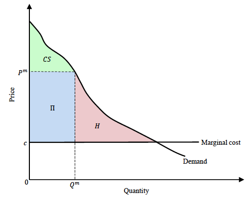
Textbook treatments such as Mankiw (2018) ascribe deadweight loss to sources such as taxes imposed by a government, or market power exercised by a monopoly. Figure 1 depicts the deadweight loss in the textbook case of a monopoly.
Figure 1 Deadweight loss in monopoly case
Source: Kremer and Snyder (2018).
The monopoly markup of price Pm above marginal cost c leaves consumers with values between the two unserved, dissipating social welfare loss amounting to the area of the triangular region H (called the Harberger triangle, after Harberger 1954).
But in a recent paper (Kremer and Snyder 2018) we argue that the deadweight loss H when the product sells at Pm can be dwarfed by the deadweight loss from the product not being developed at all. Suppose the monopolist in Figure 1 has to sink fixed cost K (R&D, capacity, advertising, or other expense) to enter the market. If the fixed cost is larger than expected profit Π, the monopolist would choose not to enter. The entire shaded region in Figure 1, not just H, would constitute unrealised social welfare.
Worst case
The maximum potential deadweight loss would be realised in the limit in which the fixed cost was slightly above the expected profit. Then the monopolist chooses not to enter, and all the social surplus in the coloured region is lost. After netting out the fixed cost, the lost social surplus equals the consumer surplus CS plus H.
The fact that the monopolist does not capture all the social benefits from its entry distorts its entry decision. These uncaptured sources of surplus – the consumer surplus flowing to high-value consumers who do purchase, and deadweight loss H dissipated from low-value consumers who do not purchase – can potentially be dissipated.
Therefore, maximum potential deadweight loss comes from the absence of a new product, not from the firm charging too high a price for it. What determines firms’ incentives to develop new products? Acemoglu and Lin (2004) point to market size: the number of consumers times their average value for the product. The larger the market, the higher the expected profit is. Higher expected profit means it would be more likely to exceed the fixed cost, inducing the firm to enter.
Worst of the worst cases
But in our paper we point to an additional factor determining entry incentives: the shape that the distribution of consumer values takes, holding the average constant.
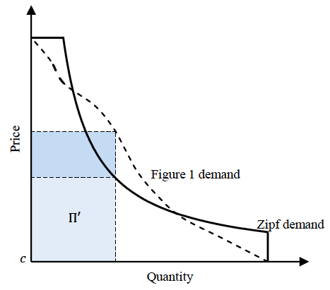
Figure 2 shows a new demand curve. It maintains the same intercept and shaded area between demand and cost as in Figure 1, but it redistributes consumer values so the monopolist earns the same profit for any price it charges, removing any sweet spot for monopoly pricing.
Figure 2 Potential deadweight loss maximised by Zipf demand
Source: Kremer and Snyder (2018).
Consumer values (net of the marginal cost c) underlying this new demand curve have a Zipf distribution – a special case of a power-law distribution with the property that consumer values are exactly inversely proportional to their rank. Monopoly profit shrinks from expected profit Π (the dark blue rectangle) to Π' (the light blue rectangle). Since the dashed and solid demand curves have the same areas underneath, maximum potential deadweight loss (equal to the area under the demand curve outside of the profit rectangle) must be larger with Zipf demand. We show the Zipf demand curve can generate the highest potential deadweight loss of any demand curve with the same area and intercepts.
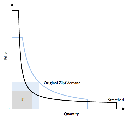
Things can get even worse. Potential deadweight loss grows as we stretch the intercepts of the Zipf demand curve, as in Figure 3, so that it hugs its boundaries more tightly. One can see that in the limit for extreme stretching, the profit rectangle disappears. Potential deadweight loss approaches 100% of social surplus.
Figure 3 Potential deadweight loss from Zipf demand grows as it stretches out along axes
Source: Kremer and Snyder (2018).
Is the worst case relevant?
This worst-worst case scenario is hardly anything to fear if it is not likely to be relevant. Unfortunately, we do not find that this is the case. As Gabaix (2009) observes, we see Zipf distributions in many economic phenomena, such as city size, firm size, CEO compensation, and wealth. These phenomena may translate into value distributions for products inheriting the Zipf shape.
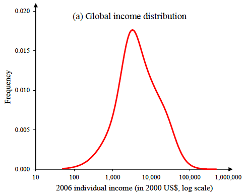
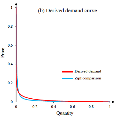
Figure 4 depicts an exercise we undertook calibrating the demand for any arbitrary product (a widget) from the most natural source we could think of – the income distribution. The exercise assumes that the widget sells on the global market. Individuals’ willingness to pay is assumed to be proportional to their income (or, in other words, their income elasticity of demand equals 1).
Figure 4 Demand derived assuming willingness to pay follows world income distribution
Source: Kremer and Snyder (2018).
The top panel of Figure 4 shows the global income distribution using data from Pinkovskiy and Sala-i-Martin (2009). Under the assumptions of the model just laid out, this income distribution generates the demand curve in the bottom panel. We were shocked to see how close the red demand curve resembled Zipf demand (the blue curve). It has the same intercepts and area underneath. In this case, a formal index of Zipf similarity that we developed equals 0.83.
Assuming that the red demand curve is served by a monopolist that has no production cost (think software, entertainment, information, or a pharmaceutical with inexpensive active ingredient), at its profit-maximising uniform price, only the richest 19% of the world population ends up purchasing. Harberger deadweight loss H equals 36% of total surplus. Maximum potential deadweight loss from the monopolist’s choosing not to produce the widget is almost double that, at 71% of total surplus.
For this deadweight loss, the fixed cost has to be a certain level (just above the area of the expected profit rectangle). Of course, we do not know what the distribution of entry costs would be for potential products to be developed in the future, but we still think there is cause for concern. The red demand curve in Figure 4 was calibrated in the most natural way we could think of, not cherry-picked to generate a bad worst-case scenario.
There is some controversy over the best estimates of the world income distribution. An alternative credible source such as Lakner and Milanovic (2016) makes a difference for poverty studies, but no difference for our measure of worst-case deadweight loss. The demand curve is still Zipf-similar in the relevant range. When production costs for the widget are moderate instead of zero, results do not change much.
Policy implications
Which policies can ameliorate this huge potential deadweight loss? If policymakers use the Zipf-similarity of demand as a criterion when targeting investment and R&D subsidies, then perhaps bigger subsidies for product innovations, or other policies with similar effects such as stronger intellectual property protections. Since the greatest potential for deadweight loss comes at the extensive (entry) margin rather than the intensive (pricing) margin, potential distortions may be greater for innovations that bring a new product to market than for process innovations that lower the cost of existing products.
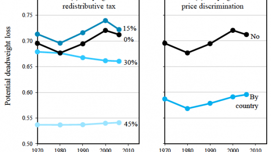
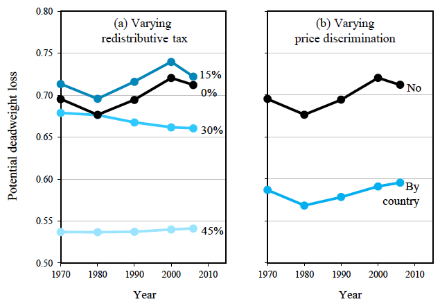
Figure 5 analyses other policies.
Figure 5 Policy impact on potential deadweight loss
Source: Kremer and Snyder (2018).
The left-hand panel looks at changing the distribution of disposable income (and thus demand curve derived from that income) via a redistributive tax. In particular, the panel supposes a proportional tax of the indicated amount is levied on all individuals, and the proceeds are redistributed to everyone in equal lump sums. The figure shows the maximum potential deadweight loss for the 2006 data (in Figure 4) but also going back to 1970. Potential deadweight loss in the baseline with no tax is drawn in black, and for various tax levels in lighter shades of blue for higher taxes.
Theoretically, if the redistributive tax is high enough, it must eventually reduce potential deadweight loss. Think about the extreme case of a 100% redistributive tax, completely levelling income. Potential deadweight loss would be eliminated by this extreme tax because the monopolist would be able to extract 100% of social surplus from the homogeneous consumers, and would have efficient entry and pricing incentives. (Consumer surplus would be eliminated as well, but that is another story.)
Surprisingly, we find a 15% tax exacerbates potential deadweight loss. Evidently, the distribution of disposable income for this tax level is more Zipf-similar than the original. Higher levels of the tax do end up reducing potential deadweight loss (somewhat by a 30% tax and more so for a 45% tax). More targeted redistributive policies (for example, redistributing all the income of those in some top percentile above the income of the top income outside of that percentile) can also be explored in this calibration.
We are not advocating particular policies in these simulations. Our toy model abstracts, among other things, from labour-supply distortion from taxation. But the simulations raise the possibility that a more egalitarian distribution of global income might encourage more product innovation.
A policy that reduces potential deadweight loss almost as effectively as the levelling effect of a 45% tax would be to allow a monopolist to price discriminate across countries (right-hand panel of Figure 5). Using the income distribution for each separate country, the optimal monopoly price and profit for each country can be computed and aggregated. The market becomes more lucrative to serve, and the deadweight loss from not entering would be reduced. For those worried about the distribution of welfare, this type of price discrimination can be implicitly redistributive, because it often results in richer nations paying far more for a good than poorer nations.
References
Gabaix, X (2009), “Power Laws in Economics and Finance,” Annual Review of Economics 1: 255–293.
Harberger, A C (1954), “Monopoly and Resource Allocation,” American Economic Review 44: 77–92.
Kremer, M and C M Snyder (2018), “Worst-Case Bounds on R&D and Pricing Distortions: Theory with an Application Assuming Consumer Values Follow the World Income Distribution,” NBER working paper 25119.
Lakner, C and B Milanovic (2016) “Global Income Distribution: From the Fall of the Berlin Wall to the Great Recession,” World Bank Economic Review 30: 203–232.
Mankiw, N G (2018), Principles of Microeconomics (8th edition), Cengage Learning.
Pinkovskiy, M and X Sala-i-Martin (2009), “Parametric Estimations of the World Distribution of Income,” NBER working paper 15433.
