Bill Phillips related changes in nominal wages to the unemployment rate as both are labour market variables (Phillips 1958). Pre-WWI data on unemployment have been substantially revised by Boyer and Hatton (2002) since the original Phillips study but our results are close to his. Phillips defined wage inflation by a two-year relative change, but we use the one-year log difference: these are highly correlated other than the timing of peaks and troughs (Hendry 2001). Variants use price inflation, measured here by the GDP deflator (Hoover 2015, provides historical perspective).
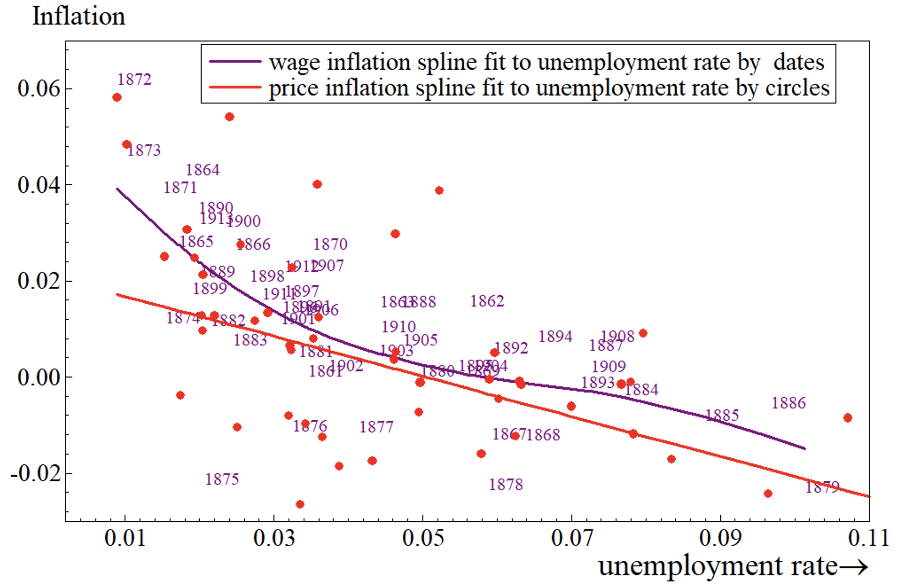
Using Phillips’ annual data from 1860 to 1913, Figure 1 compares cubic splines fitted to wage and price inflation plotted against unemployment, matching Phillips’ non-linear form, but price inflation results in a nearly straight line (purple dates are actual observations for the pairs of wage inflation and unemployment, whereas red dots are the observations for pairs of price inflation and unemployment). The wage relation was not to last.
Figure 1 Comparing the Phillips curve in price inflation with wage inflation
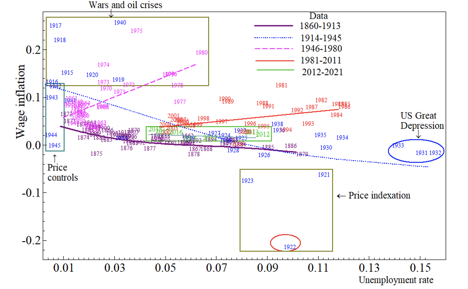
Phillips curve instability is demonstrated for the UK in Figure 2, which records five subsample estimates of the Phillips curve using annual data from 1860–2021. Every slope in sub-period relationships between wage inflation and the unemployment rate is observed, from strongly negative, slightly negative, flat, slightly positive, and strongly positive. These outcomes will be compared with those over the same sub-samples predicted by the econometric model of real-wage growth in Castle and Hendry (2014a, 2014b) (updated to 2021 in Castle et al. 2023a, 2023b), expressed in terms of nominal wage inflation.
The five sub-period plots chosen for analysis are: the original Phillips’ period, 1860–1913; WWI to the end of WWII, 1914–1945; post-war recovery until the end of the `oil crises’ 1946–1980; the sample end in Castle and Hendry (2014a, 2014b), 1981–2011; and Brexit, Covid-19 lockdowns, and the UK’s furlough scheme, 2011–2021. The ‘outliers’ from wars, oil crises, price controls, indexation, and the ‘Great Depression’ are highlighted in ‘boxes’ or `ellipses’ as deriving from different causes at different times, but don’t seem dominant. That the Phillips Curve did not fail during WWI, the inter-war period with the ‘Great Depression’, and WWII is surprising, although the downward slope estimate doubled. An upward sloping Phillips Curve during the two post-war periods, and flat since 2012, while the unemployment rate varied over 4%–8%, seem less excusable.
Figure 2 Shifts in the wage inflation-unemployment ‘trade-off’
Figure 1 showed cubic splines graphically fitted to the data as in Phillips (1958), but these are close to the linear sub-sample estimated regressions, so Table A1 in the Appendix confirms that coefficients of the unemployment rate changed substantially over time.
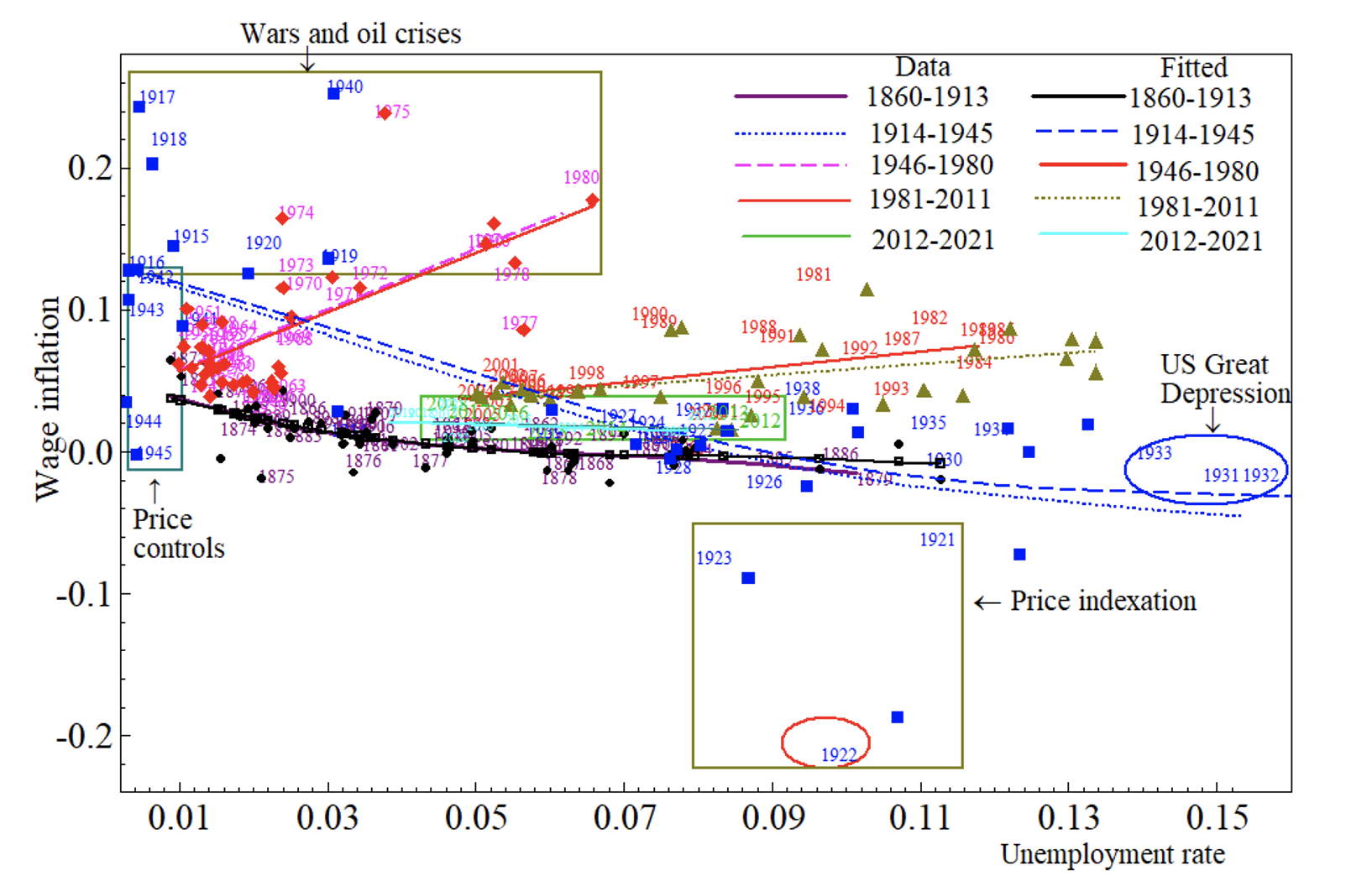
The natural explanation of unstable estimates is that relevant variables not included in the model experienced shifts. If all such excluded variables were stationary and had a constant correlation with the unemployment rate, its coefficient would be constant despite omissions. Conversely, if the additional regressors included in the econometric model of real-wage growth for 1862–2021 in Castle et al. (2023a, 2023b) embodied the shifts yet was itself constant, its sub-period predictions for nominal wage inflation should closely match. Figure 3 adds sub-period predictions from the full-sample model for nominal wage inflation against the unemployment rate. The close match confirms that the real-wage model can account for the instabilities in the Phillips curve: but which of its many variables are the culprits?
Figure 3 Comparing direct and derived Phillips curves
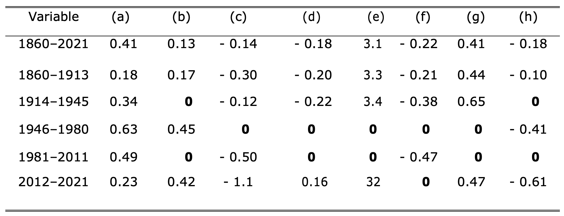
The real-wage model regressors are (a) the change in labour productivity and (b) its first lag; (c) the change in price inflation; (d) linear and (e) non-linear unemployment rates and (f) their two-period change; (g) a logistic smooth transition function interacted with price inflation for the feedback from price inflation to wages (wage-price spiral); and (h) an equilibrium adjustment from labour’s share of income lagged two periods, four step indicators and some impulse indicators. The model is constant over Brexit, the pandemic, and the UK government’s furlough scheme, and passes a test for valid conditioning of its contemporaneous regressors because the major shifts in the unemployment rate do not enter the real-wage regression. These results are consistent with the evidence in Castle and Hendry (2014a, 2014b) that most UK unemployment has been involuntary.
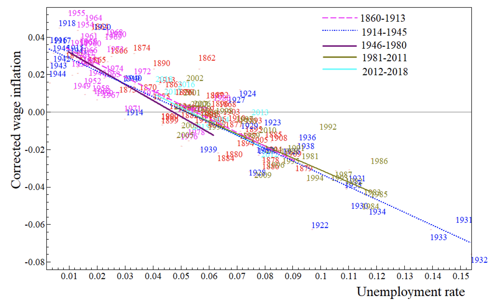
The real-wage model can be expressed as nominal wage inflation related to the unemployment rate with a unit coefficient on price inflation plus all the other variables. Summing all these full-sample influences other than unemployment, so imposing the same coefficients in all sub-periods, we regress nominal wage inflation on that scalar sum to correct it for their effects, storing the full-sample residuals (see Frisch and Waugh 1933). Then the sub-period regressions of these residuals on the unemployment rate are shown in Figure 4, and are nearly identical across all sub-periods as Table A2 in the appendix reports.
As shown in Table A3 in the appendix, the unemployment rate was uncorrelated with the cumulated sum variable on the full sample but was significantly correlated in the sub-samples where the Phillips curve shifted.
Figure 4 All sub-sample Phillips curves for nominal wage inflation on the unemployment rate corrected for the full-sample scalar
Consequently, what could have caused the shifts in the original Phillips curve sub-sample equations?
Table A4 in the appendix records significant regression coefficients from fitting the general real-wage change model to subsamples (the lettering (a)—(h) matches the explanation of the model’s variable above). Coefficients in the subsample regressions with insignificant estimates are recorded as zeroes in bold for clarity. The first two sub-periods have coefficient estimates that are relatively similar to the full sample, but the next two differ in many respects (the final sample is too short to be reliable): in particular, the impacts of the unemployment rate and its square are insignificant as are the non-linear inflation reactions. Low levels of unemployment from 1946–1980 explain its insignificance and these absent impacts on wage inflation help explain the upward slopes. Thus, the stability of the Phillips curve needed hidden co-breaking (Hendry and Massmann 2007) between the variables in the real-wage model, and the absence of some impacts stopped that occurring.
Imposing the relevant whole-sample estimates (shown in the top row of Table A3) in place of the zeroes yields an equation standard error of 1.17% for 1946–1980 versus the unrestricted sub-sample fit of 1.11%. Similarly, for 1981–2011, the restricted equation standard error is 0.91% versus 0.98%. No mis-specification tests are significant in these constrained models, consistent with the constancy of the general model despite subsample estimate variations.
Conclusion
UK Phillips curves relating nominal wage inflation to the unemployment rate are unstable with slopes that are up, down, and sideways in sub-periods over 1860–2021. But the puzzle of what caused these shifts in subsample Phillips curves is resolved as follows:
a) Mis-specification encompassing revealed that the subsample shifts could be matched by the fit of a constant parameter real-wage equation
b) Partialling out from nominal wage inflation the full-sample sum of the fitted regressors, other than the unemployment rate, revealed all the subsample equations had similar slopes in the range -0.67 to -0.85
c) Surprisingly, the unemployment rate was uncorrelated with that variable on the full sample but tests confirmed the validity and invariance of conditioning nominal wage inflation on the unemployment rate
d) Insignificance of variables in subsamples that were significant in the full-sample real-wage equation was because of little time-series variation
e) Imposing full-sample estimates on these insignificant subsample coefficients produced no deterioration in fit, identifying that the culprits behind the instability were their absence, not big shifts.
Bill Phillips and Denis Sargan debated nominal versus real wage models, so we have come full circle: the real wage equation entails a constant nominal wage model when adjusted for the same regressors. Quite a surprise that the constancy of the Phillips curve depended on co-breaking of all the variables that it omitted from the constant real-wage model which failed only when they lacked variation.
Authors’ note: Financial support from Nuffield College is gratefully acknowledged.
References
Andrews, D W K (1991), “Heteroskedasticity and autocorrelation consistent covariance matrix estimation”, Econometrica 59: 817–858.
Boyer, G R and T J Hatton (2002), “New estimates of British unemployment, 1870–1913”, Journal of Economic History 62: 643–675.
Castle, J L and D F Hendry (2014a), “Semi-automatic non-linear model selection”, in N Haldrup, M Meitz and P Saikkonen (eds.), Essays in Nonlinear Time Series Econometrics, pp. 163–197, Oxford University Press.
Castle, J and D Hendry (2014b), “The real wage-productivity nexus”, VoxEU.org, 13 January.
Castle, J L, D F Hendry and A B Martinez (2023a), “The historical role of energy in UK inflation and productivity with implications for price inflation”, Energy Economics 126 (see also the Vox column here).
Castle, J, D Hendry and A Martinez (2023b), “The role of energy in UK inflation and productivity”, VoxEU.org, 14 September.
Doornik, J A and D F Hendry (2021), Empirical Econometric Modelling using PcGive: Volume I, 9th edition, London: Timberlake Consultants Press.
Engle, R F and D F Hendry (1993), “Testing super exogeneity and invariance in regression models”, Journal of Econometrics 56: 119–139.
Frisch, R and F V Waugh (1933), “Partial time regression as compared with individual trends”, Econometrica 1: 221–223.
Hendry, D F (2001), “Modelling UK inflation, 1875–1991”, Journal of Applied Econometrics 16: 255–275.
Hendry, D F and M Massmann (2007), “Co-breaking: Recent advances and a synopsis of the literature”, Journal of Business and Economic Statistics 25: 33–51.
Hendry, D F and C Santos (2010), “An automatic test of super exogeneity”, in M W Watson, T Bollerslev and J Russell (eds.), Volatility and Time Series Econometrics, pp. 164–193, Oxford: Oxford University Press.
Hoover, K D (2015), “The genesis of Samuelson and Solow’s price-inflation Phillips curve”, History of Economics Review 61: 1–16.
Luukkonen, R, P Saikkonen and T Teräsvirta (1988), “Testing linearity against smooth transition autoregressive models”, Biometrika 75: 491–499.
Phillips, A W H (1958), “The relation between unemployment and the rate of change of money wage rates in the United Kingdom, 1861–1957”, Economica 25: 283–299.
Appendix
Table A1 Sub-period estimates of the unemployment rate coefficients from wage inflation regressions, with heteroscedasticity and autocorrelation consistent (HAC) standard errors (Andrews 1991)
Table A2 Coefficient estimates for the unemployment rate in the subsample real-wage regressions with HAC standard errors
Table A3 Coefficient estimates, standard errors and fit measured by the equation standard error of the sub-sample regressions of the unemployment rate on the full-sample scalar
Table A4 Coefficients in the subsample regressions of the real-wage change model with absolute `t’ statistics greater than 2

