Behavioural economics is seeing increased acceptance as a legitimate way of thinking about economic issues. The recent awarding of the Nobel Prize to Richard Thaler testifies that there has been a change of view within the economics profession on the need to allow for departures from the paradigm of the ‘homo economicus’.
This is much less the case in mainstream macroeconomics, however. Homo economicus continues to reign supreme in dynamic stochastic general equilibrium (DSGE) models. In these models, individual agents maximise an infinite horizon utility function using rational forecasts based on all available information including the information embedded in the model. Nothing really can go wrong in models populated by supreme agents peacefully optimising and endowed with great cognitive abilities that allow them to understand the complexities of the world. Only exogenous disturbances can get these agents off the rail, forcing them to re-optimise. These models then lead to the view that business cycle fluctuations occur as a result of exogenous events (shocks) that force individuals to reconsider their optimal plans. Nothing in the model creates endogenous business cycle movements. Booms and busts are all the result of exogenous disturbances (Smets and Wouters 2007, Gali 2008).
‘Behavioural’ macroeconomic models
We need to do better – and that is what we have been trying to do in a series of publications (De Grauwe 2012, De Grauwe and Corrado 2015, De Grauwe and Ji 2016, 2017a). We are, of course, not alone in exploring different tracks of macroeconomic modelling. There is a growing number of researchers developing ‘agent-based’ models and ‘behavioural’ macroeconomic models (Alfarano et al. 2005, Tesfatsion and Judd 2006, Colander et al. 2008, Farmer 2006, Farmer and Foley 2009, Gatti et al. 2011, Gabaix 2014, Westerhoff and Franke 2012, Hommes 2016, Hommes and Lustenhouwer 2016, Muellbauer 2017; see also the recent criticism of Blanchard 2017 and the chapters in Gürkaynak and Tille 2017).
There are many ways in which one can depart from mainstream macroeconomic models. We have chosen to do so by assuming that agents experience cognitive limitations preventing them from having rational expectations. Instead, these agents use simple forecasting rules (heuristics) and evaluate the forecasting performances of these rules ex post. This evaluation leads them to switch to the rules that perform best. It can be argued that in a world of great complexity that nobody fully understands, such a process of adaptive learning might be the rational way of deal handling this complexity (Simon 1957, Gigerenzer and Selten 2002, Ackerlof and Shiller2009).
This adaptive learning assumption introduced in an otherwise standard New Keynesian macroeconomic model produces endogenous waves of optimism and pessimism (animal spirits) that drive the business cycle in a self-fulfilling way. This also leads to a two-way causality. That is, optimism (pessimism) leads to an increase (decline) in output, and the increase (decline) in output in term intensifies optimism (pessimism) (De Grauwe 2012, De Grauwe and Ji 2017a).
An important feature of this dynamics of animal spirits is that the movements of the output gap are characterised by periods of tranquility alternating in an unpredictable way with periods of intense movements reflecting booms and busts. Technically, this means that the distribution of the output gap and output growth is non-Gaussian and exhibits fat tails.
There is now a significant body of empirical evidence showing that the output gaps (and also the growth of output) in OECD countries do not exhibit a Gaussian distribution, but are characterised by excessive kurtosis and fat tails. Fagiolo et al. (2008) and Fagiolo et al. (2009) carried out important econometric analysis documenting the non-normality of the distribution of output gaps and growth rates of GDP. Thus, our behavioural model predicts that in the real world the output gap does not follow a normal distribution, but is characterised by excess kurtosis and fat tails. This feature of the higher moments of the output gap is generated endogenously in the model. It is not the result of imposing such a feature on the stochastic shocks hitting the economy.
The contrast with standard DSGE-models is significant. These models find it difficult to explain the fat tails in the distribution of the output gap. They have to rely on large exogenous shocks as explanations of the boom and bust features of business cycles. Such an explanation is not satisfactory, as it shifts the burden of explaining the business cycle to outside forces. One good example is the recent effort to integrate the financial sector in DSGE models to explain the business cycle. However, the results of these models depend on the assumption that the shocks are serially-correlated. As a result, one can argue that standard DSGE models do not have an endogenous business cycle theory.
Applying our model: How structural reforms affect the nature of business cycles
We have used our behavioural macroeconomic model to analyse different macroeconomic issues. One issue is the high synchronisation of national business cycles in the industrialised world. These cannot be easily explained in standard macroeconomic models except by (again) assuming common exogenous shocks. We extended our behavioural model to two countries and found that the model is capable of generating a strong international transmission of animal spirits, which in turn leads to a strong correlation of business cycles. These come close to the observed correlations. We achieve this without the need to invoke common exogenous shocks (De Grauwe and Ji 2016).
In our latest paper, we used the same behavioural model to analyse how structural reforms affect the nature of business cycles, and the capacity of the central bank to stabilise output and inflation (De Grauwe and Ji 2017b).
We introduce structural reforms in the context of this behavioural model through two channels. The first is through the sensitivity of inflation to the output gap in the New Keynesian Philips curve (supply equation). A low sensitivity of the rate of inflation with respect to the output gap is indicative of wage and price rigidities.
The second way we introduce structural reforms is through changes in the supply equation. This is also the way structural reforms have been modelled in standard DSGE models (e.g. Eggertson et al. 2014, Cacciatore et al. 2012, Everaert and Schule 2006, Gomes et al. 2013, ECB 2015). In these models, structural reforms in labour markets include relaxing job protection, cuts in unemployment benefits, and so on; in product markets the reforms include reductions in barriers to entry for new firms. These reforms lead to a lowering of mark ups in the goods and labour markets and move the economy closer to perfect competition. Therefore, these reforms can be seen as shifting the supply curve to the right, increasing the production potential of countries.
We find that structural reforms that increase the flexibility of wages and prices can have profound effects on the dynamics of the business cycle. In particular, in a more flexible economy (more wage and price flexibility), the power of animal spirits is reduced and so is the potential for booms and busts in the economy. This has to do with the fact that in more flexible economies prices and wages have a greater role to play in adjustments to emerging disequilibria. This reduces the amplitude of business cycles, and as a result creates less scope for waves of optimism and pessimism in creating booms and busts.
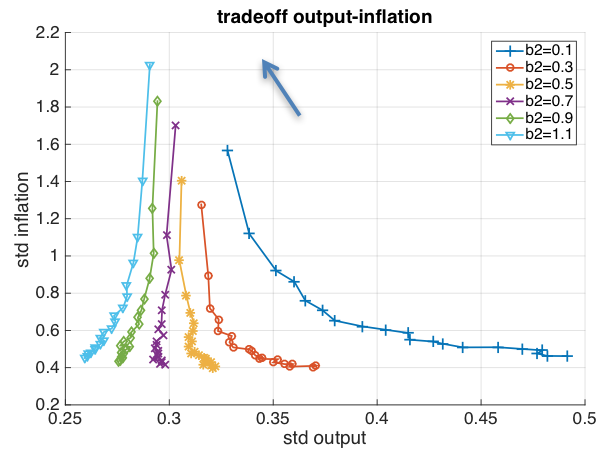
The major question we analyse is how structural reforms affect the choices monetary authorities face. In order to do so, we constructed policy trade-offs of the central bank for different levels of flexibility. The latter is measured by the sensitivity of inflation to the output gap in the New Keynesian Philips curve (called b2). The trade-offs are represented in Figure 1. These measure the inflation and output volatility choices the central bank faces when it increases its inflation control (measured by the sensitivity of the interest rate to changes in inflation in the Taylor rule).
In order to understand Figure 1 let us first concentrate on the case of low flexibility (b2 = 0.1). In this case, the trade-off is negatively sloped. Starting from the top of that trade-off, we see that increasing the inflation control (measured by the inflation parameter c1 in the Taylor rule) leads to a decline of inflation volatility at the expense of more output volatility. As the degree of flexibility increases, we observe that the trade-off curves shift to the left and become less negatively sloped. For values of b2 exceeding 0.5, these trade-offs become positively sloped – that is, when c1 (the inflation parameter in the Taylor rule) increases, both inflation and output volatility decline.
Thus, one can conclude that when the economy is very rigid, a central bank that pursues its inflation target with increasing intensity faces a classical negatively sloped trade-off between inflation and output volatility. This trade-off disappears when the economy is sufficiently flexible. In that case, the central bank can pursue a tighter inflation target without paying a price in terms of a higher output volatility. Put differently, in a flexible economy, attempts by the central bank to better stabilise inflation are welfare improving. This is not so when the economy is too rigid.
Figure 1 Trade-off between output and inflation
This may lead to the conclusion that flexibility is always welfare improving – but that is not the case. In fact, we can see from Figure 1 that the positively sloped ‘trade-offs’ move upward and to the left (indicated by the arrow) for increasing levels of flexibility (b2). This means that if the central bank keeps its inflation control unchanged, increasing flexibility creates a new trade-off, which is negatively sloped – that is, more flexibility then reduces output volatility at the expense of more inflation variability.
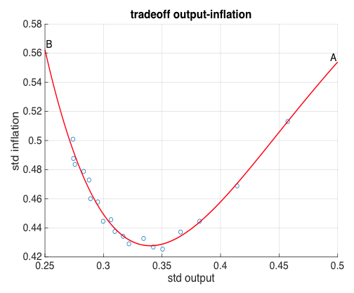
This insight allows us to derive this new trade-off by connecting the points that are associated with the same inflation parameter of the Taylor rule. We show the result for a given c1 = 1.5 (the inflation parameter) and c2 = 0.5 (the output parameter) in Figure 2. This presents the relationship between output and inflation variability that we obtain for increasing levels of flexibility, assuming that the central bank keeps its inflation control constant. The horizontal axis shows the standard deviations of output; the vertical axis the standard deviations of inflation. We obtain a non-linear relationship. In order to understand this, start from point A. This point is obtained when flexibility is zero (i.e. wages and prices do not react to changes in the output gap). As we increase the degree of flexibility, we move down along the downward sloping segment of the line. This downward movement implies that increasing flexibility creates a ‘win-win’ situation in that both the volatility of output and inflation decline with increasing flexibility. Put differently, as we move down from point A there is an unambiguous increase in welfare. However, when we go too far with structural reforms, we go beyond the minimum point on the line. From that point on, we obtain a negatively sloped relationship (i.e. further increases in flexibility lead to less volatility of output at the expense of increasing inflation volatility).
Figure 2 The optimal level of flexibility
Figure 2 allows us to obtain some insights about the optimal level of flexibility. Clearly, this must be located to the left of the minimum point of the relationship. Any point on the positively sloped part can be improved upon by increasing flexibility. Beyond the minimum point further increases in flexibility lead to lower output volatility at the expense of higher inflation volatility. Where the optimum flexibility will be reached then depends on the preferences about inflation versus output volatility.
Concluding remarks
We conclude that the degree of flexibility has profound effects on the trade-offs central banks encounter in their attempts to stabilise the economy. In general, in more flexible economies central banks do not face the same kind of uncomfortable trade-offs as in rigid economies. No wonder, then, that central banks like structural reforms that increase the flexibility of the economy. We also found, however, that there is a limit to the comfort flexibility can provide to central bankers.
References
Akerlof, G and R Shiller (2009) Animal spirits: How human psychology drives the economy and why it matters for global capitalism, Princeton University Press.
Alfarano, S, T Lux and F Wagner (2005), “Estimation of agent-based models: The case of an asymmetric herding model”, Computational Economics 26: 19–49.
Blanchard, O (2017) “Do DSGE models have a future?” in R Gürkaynak and C Tille (eds), DSGE Models in the Conduct of Policy: Use as Intended, VoxEU ebook.
Cacciatore, M, R Duval and G Fiori (2012) “Short-term gain or pain? A DSGE model-based analysis of the short-term effects of structural reforms in labour and product markets”, OECD, Economics Department Working paper no 948.
Colander, D, P Howitt, A Kirman, A Leijonhufvud and P Mehrling (2008), "Beyond DSGE models: Toward an empirically based macroeconomics", American Economic Review 98(2): 236-40.
De Grauwe, P (2012) Lectures on Behavioural Macroeconomics, Princeton University Press.
De Grauwe, P and C Macchiarelli (2015) “Animal spirits and credit cycles”, Journal of Economic Dynamics and Control 59: 95-117.
De Grauwe, P and Y Ji (2016), “International correlation of business cycles in a behavioural macroeconomic model”, CEPR, Discussion Paper, April.
De Grauwe, P and Y Ji (2017a) “Inflation targets and the zero lower bound in a behavioural macroeconomic model", Economica, forthcoming.
De Grauwe, P and Y Ji (2017b), “Structural reforms and monetary policies in a behavioural macroeconomic model", CEPR, Discussion Paper no 12336.
Delli Gatti, D, C Di Guilmi, E Gaffeo, G Giuloni, M Gallegati and A Palestrini (2005), “A new approach to business fluctuations: Heterogeneous interacting agents, scaling laws and financial fragility”, Journal of Economic Behavior and Organization 56: 489-512.
Eggertsson, G, A Ferrero and A Raffo (2014), "Can structural reforms help Europe?" Journal of Monetary Economics 61: 2-22.
Evans, G and S Honkapohja (2001), Learning and Expectations in Macroeconomics, Princeton University Press.
Farmer, R E A (2006), “Animal Spirits”, Palgrave Dictionary of Economics.
Farmer, R, J Doyne and D Foley (2009), “The economy needs agent-based modelling”, Nature 460: 685-686
Gabaix, X (2014), “A sparsity-based model of bounded rationality”, The Quarterly Journal of Economics, 1661–1710.
Galí, J (2008), Monetary policy, inflation and the business cycle, Princeton University Press.
Gigerenzer, G and R Selten (2002), Bounded rationality, Cambridge: MIT Press.
Gürkaynak, R and C Tille (2017), “DSGE models in the conduct of policy: Use as Intended”, VoxEU.
Hommes, C (2016), “Behavioural macroeconomics with heterogeneous expectations and interacting agents”, Discussion Paper, CenDEF, University of Amsterdam.
Hommes, C and J Lustenhouwer (2016), “Managing heterogeneous and unanchored expectations: A monetary policy analysis”, Working Paper, Tinbergen Institute, Rotterdam.
Muellbauer, J (2016), “Macroeconomics and consumption”, CEPR Discussion paper 11588; Oxford University, Department of Economics working paper 811.
Simon, H (1957), "A behavioural model of rational choice", in Models of Man, Social and Rational: Mathematical Essays on Rational Human Behavior in a Social Setting, New York: Wiley.
Smets, F and R Wouters (2007), “Shocks and frictions in US business cycles: A Bayesian DSGE approach”, American Economic Review 97(3): 586–606.
Tesfatsion, L and K L Judd (2006), Handbook of Computational Economics Volume 2: Agent-Based Computational Economics, Elsevier.
Westerhoff, F and R Franke (2012), “Agent-based models for economic policy design: Two illustrative examples”, Iowa State University, Working Paper No 88.


