The Great Recession of 2007-2009 was the major macroeconomic downturn of the postwar period. It happened when several measures of household inequality were at a postwar high. Is there a connection between these two observations? Did the high level of household inequality amplify and propagate the Great Recession? How are the welfare losses in an economic downturn, such as the 2007-09 crisis, distributed across households, and can social insurance policies mitigate these losses?
In a well-known paper published in 1998, Krusell and Smith concluded that household income and wealth inequality had little impact on the aggregate dynamics of consumption, investment, and output. Their model economy had heterogeneous agents and incomplete markets, and it behaved much like a model that used a representative household. This result has reinforced the continued use of representative agents when studying the macroeconomy.
In a recent study, we revisited the importance of household heterogeneity for aggregate consumption and output dynamics (Krueger et al. 2016a). Unlike Krusell and Smith, we found that inequality has a significant impact on business cycle fluctuations. In other words, we find that micro heterogeneity is important for macro outcomes We also explored (Krueger et al. 2016b) how large downturns differentially impact household welfare depending on wealth, employment, and how social insurance affects those welfare losses. We find that the macro shocks can have a sizeable impact on household welfare and one that is different across the wealth distribution, in other words, macro dynamics are important for micro outcomes.
Wealth inequality and consumption rate
Table 1 shows some key facts about the US income, wealth and consumption distribution in 2006, just before the great recession. It is taken from the Panel Study of Income Dynamics (PSID), a household survey that has been running since 1968. It collects information about household wages, labour market outcomes, wealth, and comprehensive measures of household consumption expenditures. To construct the table, we sorted households by wealth measured as net worth (the value of all households assets, financial and real, including the value of a household’s home, subtracting all household liabilities such as mortgage debt). We report the share of economy-wide net worth owned by households in each of the five quintiles of the wealth distribution.
The third and fourth columns summarise the share of disposable income and consumption for households at different points of the wealth distribution. The last column calculates the expenditure rate by wealth quintile, measured as the ratio of total consumption expenditure to total disposable income for each quintile.
Table 1 Distribution of wealth, income and consumption by wealth quintile
Source: PSID.
Clearly, wealth is extremely unequally distributed in the US. The bottom 40% of households hold no net worth at all, while the upper 20% hold 83% of total net worth. The highest wealth quintile holds a disproportionate share of aggregate income and consumption too.
But despite holding virtually no wealth, the bottom 40% of households still account for close to 25% of aggregate consumption. As the last column of Table 1 shows, households at the lower end of the wealth distribution consume a larger share of their disposable income. Therefore, we would expect their expenditures would to respond more strongly to a large and prolonged economic downturn.
Did household inequality amplify and propagate the Great Recession?
To investigate this, we constructed a standard macroeconomic model with aggregate shocks and household heterogeneity in incomes and preferences, using Krusell and Smith's method. But we ensured that our model had cross-sectional wealth and consumption distributions that replicate the PSID data. In our model, highly persistent income shocks, coupled with unemployment insurance, mean the bottom 40% in the model held no wealth, but made up a significant share of consumption. A group of especially patient households made up the top of the wealth distribution, and accounted for approximately 80% of all wealth in the economy.
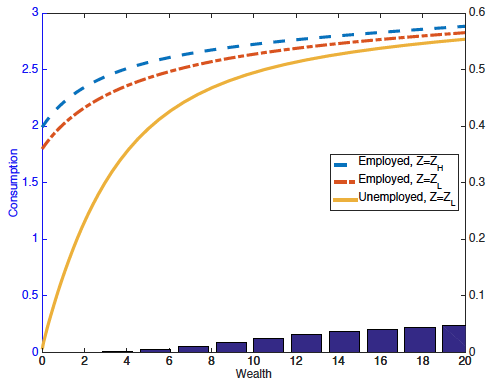
We then subjected our model economy, as well as an economy with much greater wealth equality, to the same large negative shock. This was a drop of total factor productivity of 4% relative to trend, expected to last 22 quarters. For the model with 2006-like wealth inequality, compared to an economy with little or no wealth inequality, the consumption expenditure recession on impact is half a percentage point larger, representing about $200 per capita,. Figure 1 illustrates this.
Figure 1
This figure displays the consumption functions and wealth distributions from two models. 'KS' is based on the model economy studied by Krusell and Smith. It allows only limited wealth inequality. On the other hand, our model's cross-sectional wealth distribution in 2006 is consistent with that in the data. The left-hand panel shows the KS economy, with consumption functions (plotted against individual wealth on the horizontal axis) for three combinations of idiosyncratic employment and aggregate productivity states. For a given wealth level, the vertical difference between the consumption functions for the employed in aggregate state Z = Zh (the blue dashed line) and the employed in aggregate state Z = Zl (the red dot-dashed line) gives the consumption drop in the Great Recession, conditional on not losing a job. In the same way, the vertical distance between the blue-dashed consumption function and the orange solid consumption function (for the unemployed in the recession) gives the consumption decline for those households that lose their jobs. The figure also shows the pre-recession wealth distribution, displayed as a histogram.
The right-hand panel displays the same information, but for an economy that uses 2006 data.
For a given level of wealth we can see that the drop in individual consumption in the KS economy in the Great Recession would actually have been larger than in the benchmark economy. This is mainly because the benchmark economy has a more generous unemployment insurance system that stabilises individual consumption. This is especially true for households with little wealth that lose their jobs at the onset of the recession.
These larger individual consumption declines in the KS economy might suggest that the aggregate consumption recession is also larger for the KS economy than for the 2006 benchmark economy. This is not so. In the KS economy, the cross-sectional wealth distribution places almost no mass on households with very little net worth. In contrast, the benchmark model with realistic wealth inequality has many households at zero or close to zero wealth. For these households, the individual consumption losses are significant. This is especially true for newly unemployed households. Therefore the aggregate consumption recession is significantly larger when the bottom 40% of the population has close to zero wealth than in a more equal distribution.
We would like to stress that the reason why the aggregate drop in expenditures is much larger in the economy with many low wealth consumers is not driven by the fact that low wealth households are ‘hand-to-mouth’ consumers, who cut their expenditure one-for-one as their income falls. It is instead explained by the fact that low-wealth consumers have a lesser ability to self-insure against idiosyncratic risk, so when the recession hits and unemployment risk increases, they drastically reduce their expenditure rates, even if their income has not dropped yet. Interestingly this is a prediction of the model, but is also observed in the PSID data. For example, in our work we document that over the course of the Great Recession, households in the bottom quintile of the wealth distribution reduced their expenditure rates by roughly 4 percentage points, while those in the top quintile only cut their expenditure rates by 2 percentage points.
How are the welfare losses in an economic downturn distributed?
The size of a public unemployment insurance (UI) programme affects the wealth distribution, but also the size of the individual consumption decline in a recession for a given wealth level. Holding the wealth distribution constant, a less generous system of UI (a reduction of the UI replacement rate from 50% to 10% in this case) amplifies the aggregate consumption recession by two percentage points. When the wealth distribution responds to the policy change, three quarters of this amplification disappears.
Figure 1 showed that the decline in individual consumption in the Great Recession would have differed strongly among households depending on their wealth levels and whether they lost their job. It therefore is likely that the welfare losses were unevenly distributed across the US population, and shaped by the size of social insurance programs such as UI.
In the second part of our research, we showed that this is indeed the case (Krueger et al. 2016b). Using the same set-up described above, we tried a thought experiment: what share of lifetime consumption would a household be willing to give up to avoid seeing the macroeconomy slip into a 2006-style 'great recession'?
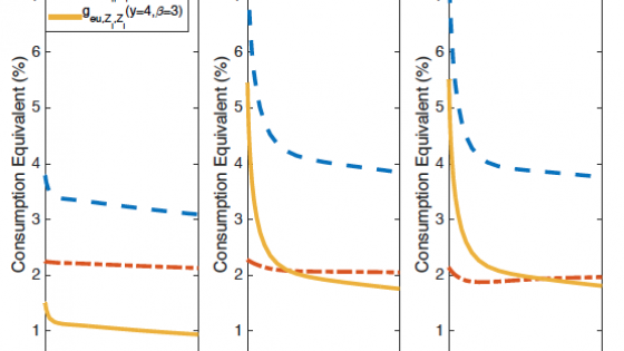
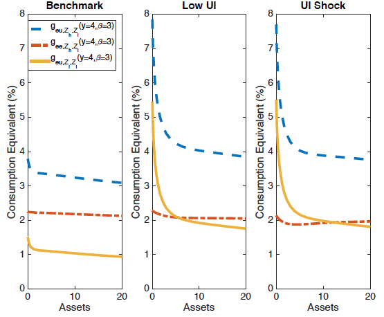
Figure 2 summarises the results. The three panels differ according to the size of the UI system: a replacement rate of 50% in the left-hand panel, a replacement rate of 10% in the middle panel, and a surprise reduction of the UI replacement rate at the time of a great recession from 50% to 10% (think of UI benefits unexpectedly running out) in the right-hand panel. Each panel plots welfare losses from the economy falling into a great recession (red dashed line), losing one’s job (orange solid line) and the combination of both events, against wealth.
Figure 2
We observe that these welfare losses are large (up to 8% of lifetime consumption), substantially larger if the UI system is small, and significantly larger for households with little wealth. If UI benefits are generous (see the left-hand panel) the aggregate component of the welfare losses is larger than the idiosyncratic component of losing one’s job. Primarily this is because future unemployment risk goes up in aggregate downturns – even for households that have not yet lost their jobs, and we attribute this added unemployment risk to the aggregate welfare loss component. In the benchmark economy with realistic wealth inequality, aggregating across households, the welfare losses from the great recession were 2.2% of lifetime consumption; in the economy with limited wealth dispersion the losses were only 1.6%. This was mainly because the KS economy has few people with little wealth, and it is these households that suffer the most from experiencing a great recession.
Taking both of our papers together, we conclude that measuring and modeling household heterogeneity explicitly is of crucial importance in macroeconomic research for two reasons.
- The first is that macroeconomic dynamics are affected by the degree of underlying heterogeneity. In particular, an economy with a large fraction of low-wealth households will experience a sharper reduction in aggregate consumption expenditures in response to a given macroeconomic shock.
- The second reason is that, in terms of welfare, the impact of a given macroeconomic shock is felt very differently in different segments of the wealth distribution. In particular, low-wealth households have limited capacity to insure themselves against idiosyncratic risk, and thus the welfare impact of a recession is significantly larger for them. As a consequence, ignoring wealth heterogeneity can severely underestimate the welfare cost of a large recession.
References
Krueger, D., Kurt Mitman and F. Perri (2016a), "Macroeconomics and Household Heterogeneity", CEPR Discussion Paper No. 11038.
Krueger, D., Kurt Mitman and F. Perri (2016b), "On the Distribution of the Welfare Losses of Large Recessions", CEPR Discussion paper 11413.
Krusell, P. and A. Smith (1998), Income and Wealth Heterogeneity in the Macroeconomy, Journal of Political Economy, 106, 867-896.


