Editor's note: This column first appeared as a chapter in the Vox eBook, The Long Economic and Political Shadow of History, Volume 1, available to download here.
Why do people, in the world as a whole or within a given country, live where they do? Why are some places so densely populated and some so empty? In daily life, we take this variation in density as a matter of course, but in many ways it can be quite puzzling.
Economists point to three factors to explain how population is distributed. The first is that there are differences in geographical characteristics, often referred to as ‘first nature’, that make some places better disposed for habitation or producing output than others. This explains why mountainous regions, deserts, tundra and so on tend to have low population density, and why much of the world’s population is situated in places where it is relatively easy to produce food.
The second factor is agglomeration. Because of economies of scale and gains from trade, we humans often find it efficient to gather in small areas. Of course, many industries, most notably food production, don’t benefit from such concentration, and are instead spread out in accordance with the availability of first nature resources. Further, there are limits to the benefits of agglomeration: because of congestion and transport costs, the urban population is spread among many cities, which are, in turn, spatially dispersed.
The final factor affecting the distribution of population is history. Cities, once established, have a very strong tendency to stay put. This persistence results from many factors, often collectively described as ‘second nature’ (Cronon 1992). Among these factors are long-lived capital, political power, and the fact that once agglomeration has started in a particular place, it will be a natural focus for future equilibria. As discussed by Bleakley and Lin (2012) and Michaels and Rauch (forthcoming), this persistence can be important, even when the reasons that a city has been established in a particular place are no longer important.
The complete story of how nature, agglomeration, and history have interacted to give the world the distribution of population that we see today is far too complex to be captured in a single study. The goals in our recent paper are less ambitious (Henderson et al. 2017). We ask how economic and technological development have changed the ways in which first-nature characteristics impact population distribution. While these characteristics themselves haven’t changed too much over history (so far), the way in which they affect settlement has. Simple examples of such changes are the impacts of air conditioning, irrigation, and the discovery of new uses for particular mineral resources. We focus on the two natural characteristics where we think that changes associated with economic and technological change have been most important. These are, first, the suitability of a region for growing food, and second, the suitability of a region for engaging in national and international trade. Over the last several centuries, the importance of fertile land as a determinant of population density has declined, both because agricultural productivity has increased – so that a smaller fraction of the labour force works on farms – and because transport costs have fallen – so that people don’t need to live near where their food is produced. Lower transport costs, along with increased opportunities for gains from trade, have similarly raised the value of locations (such as those on coasts, navigable rivers, or natural harbours) that are accessible to trade, either within or between countries.
Our goal is to show how these changes are reflected in the distribution of population today. In pursuing this goal, the effect of persistence, as described above, turns out to be very important. We are interested in how technology in historical times affected agglomeration at those times, but the data on population density that we use (described below) is only available for the world today. However, if we know when (in a rough sense) agglomeration began in a country, then we can use the similarity of today’s distribution to the historical distribution to learn about how the technology available at that time affected agglomeration.
First-nature data and the distribution of population today
Before looking at the role of history, we start by simply examining the explanatory power of first-nature characteristics for population distribution in the world today, which is arguably an interesting issue in its own right.
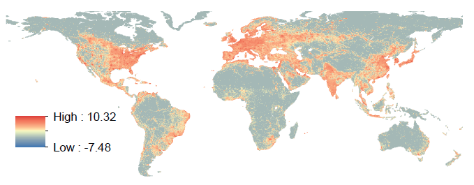
Our starting point, in measuring the dispersion of population, is lights observed at night by weather satellites. Specifically, we use the 2010 Global Radiance Calibrated Nighttime Lights dataset (Ziskin et al. 2010). In previous work (Henderson et al. 2012), we showed that change over time in night-lights data is a useful proxy for the growth of GDP in countries with poor national income accounts data. The lights data are distributed as a grid of pixels of dimension 0.5 arc-minute resolution (1/120 of a degree of longitude/latitude). We aggregate into a grid of 1/4-degree squares, with each square covering approximately 770 square kilometres at the equator. At this resolution our sample is roughly 240,000 grid squares (excluding squares made up solely of water). Figure 1 shows this grid cell data for the world as a whole.
Figure 1 Demeaned lights
The first-nature variables we use in predicting lights come in three groups. The first, labelled ‘agriculture’, are factors that seem clearly related to producing food. These comprise six continuous variables (temperature, precipitation, length of growing period, land suitability for agriculture, elevation, and latitude) as well as a set of 14 indicators for biomes (mutually exclusive regions, encoding the dominant natural vegetation expected in an area, based on research by biologists.) The second group of variables, labelled ‘trade’, focus on access to water transport. These are dummy variables for whether the centre of a grid cell is within 25 kilometres of a coast, navigable river, major lake, or natural harbour, as well as a continuous measure of distance to the coast. Finally, we define a ‘base’ group of two variables – ruggedness and malaria ecology – which seemed to us to be roughly equally relevant for agriculture and trade.
Figure 2a Demeaned predicted lights without fixed effects
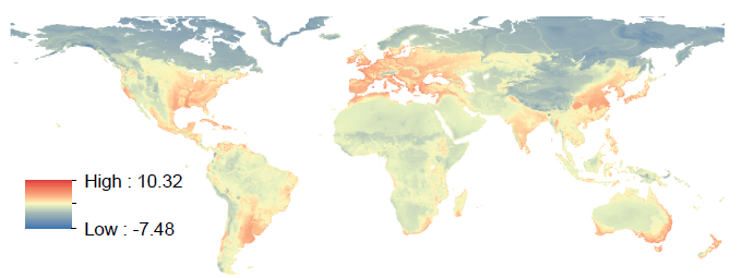
Figure 2a shows the fitted values from regressing lights in a grid square on our three sets of first-nature variables. Together, these variables explain 47% of the variation in lights and, looking at the figure, there is clearly a strong resemblance between the fitted values and the world as we know it. However, there are two potential problems associated with jumping from this result to the conclusion that nature really does explain such a large fraction of variability in population density. The first is that variation in visible light is not solely determined by population density. The other big determinant is income per capita. It is for this reason that, in Figure 1, Japan is so much brighter than Bangladesh, even though the latter is more densely populated. The second problem is that a statistical correlation between geographical characteristics and either income or population density might not indicate a true effect of geography, but rather be proxying for the effect of something correlated with geography. For example, if European colonisers implanted good institutions in places where the climate was amenable to their settlement, and bad institutions in places where it was not (the story of Acemoglu et al. 2001), then a European-type climate will predict higher income, even though it may not directly affect income at all.
Figure 2b Demeaned predicted lights with fixed effects
Both of these problems are addressed by looking at variation in lights and natural characteristics within countries. Formally, this amounts to including country-fixed effects in our analysis, which is done in all the work reported below. Figure 2b is an example of this: we estimate the effect of first-nature characteristics, using only within-country variation in lights, and then form fitted values for the world as a whole, omitting the estimated country fixed effects. As the figure shows, knowing only how geography affects population within countries, one would still do a pretty good job of predicting the variation in population density the world over. The agriculture and trade variables account for slightly more than one-third of within-country variation.
The changing importance of first-nature characteristics
We now turn to the question of how the importance of natural characteristics, as a determinant of the distribution of population, has changed over time. As mentioned above, a key to our approach is comparing countries where agglomeration took place early, thus reflecting the weights put on natural characteristics further back in time, with those that agglomerated later. Unfortunately, we don’t have a good, consistent measure of exactly when agglomeration took place, so instead we use data from 1950, on both urbanisation as well as two proxies: education and GDP per capita. Our assumption is that countries with higher values of these measures, as of that point in time, also started their urbanisation process earlier. We use several statistical approaches to parse the data. One is to estimate coefficients on our ‘agriculture’ and ‘trade’ variables separately for early and late agglomerators, while simultaneously letting the data determine where the cutoff is between these two groups of countries (essentially, looping through all possible division points to find the one that gives the best fit). Applying this method, using urbanisation in 1950, for example, we find that the cutoff between early and late agglomerators is an urbanisation rate of 36.2%, which puts 70 out of 189 countries (57.2% of our grid squares) in the ‘early’ category. Table 1 then shows the R-squareds from running regressions of visible lights on either the set of base variables (including country fixed effects), the base plus agriculture variables, or the base plus trade variables. The improvement in fit that comes from adding agricultural variables is much larger in the early than in the late agglomerating countries; correspondingly, the improvement in fit that comes from adding trade variables is much larger in the late agglomerating countries than in the early agglomerators. We find a similar pattern when we use education or GDP per capita in 1950 to split the data, and we find it also when we look solely within the New World or the Old World. We also find similar results when we look at other specifications, for example linearly interacting urbanisation or its proxies with agriculture and trade variables.
Table 1 R-squareds
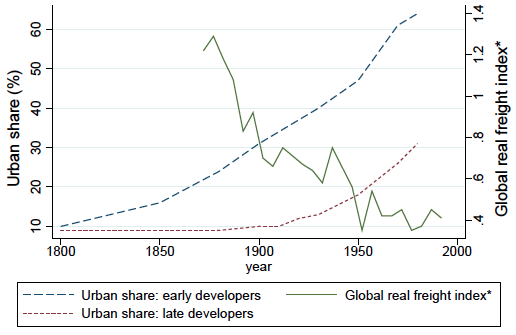
These results tell what, at first, seems to be a puzzling story: late agglomerators are generally poorer countries, and on average are more dependent on agriculture than early agglomerators. Yet it is in the latter group of countries that agricultural variables do a better job of predicting the location of population and economic activity. Our explanation of this apparent puzzle looks to the timing of when agricultural productivity rose and similarly when trade costs fell. In countries where agglomeration got going early, the rise in agricultural productivity preceded the decline in transport costs. That is, people began moving from farms to cities at a time when it was still relatively expensive to move food from place to place. As a result, cities were located close to areas conducive to food production. By contrast, in late agglomerators, the rise in agricultural productivity that allowed urbanisation came later, relative to declining transport costs, and so the latter was relatively more influential as a determinant of location. Figure 3 shows some of the data that supports this story: it plots the urban share of the population in groups of early and late agglomerators, as well as a global index of transport costs. The figure makes clear that transport costs were far lower when late agglomerators reached any particular level of urbanisation than when the same level was reached by early agglomerators.
Figure 3
Note: *excludes periods including world war years
Sources: Bairoch (1988); Mohammed and Williamson (2004)
An interesting implication of this analysis is that countries that are only urbanising now have population distributions that are more appropriate to modern technology than do those that urbanised earlier. For example, even though, in Europe, coastal areas already have particularly high population densities, our estimates imply that, had Europe developed later, coastal density would be even greater. Similarly, had Africa developed earlier, interior areas such as the Ethiopian highlands and the Congo basin would have higher relative population densities than those actually observed today.
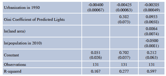
Another set of implications, drawn from the story in our paper, involves spatial inequality within countries. We expect that early agglomerators, with their activity focused around agriculturally suitable land, and a distribution of population inherited from a period when transport costs were high, should have a higher degree of spatial equality in lights overall than late agglomerators, with their heightened coastal focus and low transport costs. To assess this prediction, we calculate a spatial Gini coefficient for light across grid cells for each country. Table 2 shows the results from regressing the lights Gini on urbanisation in 1950. The coefficient is negative, as predicted. Further, controlling for the Gini of lights predicted using our geographic variables, as well as measures of country size and population (and thus population density), does not affect the result.
Table 2 Gini coefficient of lights
Conclusion
The saying that “geography is destiny” is often attributed to Napoleon. Meanwhile, the American industrialist Henry Ford really did say that “history is bunk.” In our research, we have shown that, when it comes to thinking about how population is distributed within countries, there is reason to doubt both of these statements. Geography clearly matters quite a bit, when it comes to where people live. But the aspects of geography that matter change over time. Further, there is enormous persistence in location, so that the ways in which geography mattered in the past – that is, history – are still reflected in the spatial distribution of population today.
To many readers, sitting in cities founded hundreds of years ago, sipping coffee grown thousands of kilometres away, none of this will come as a great surprise. However, understanding the dynamic interplay of geography, technology, economic growth, and history – a project in which our paper is only a small step – is of great import in thinking about many issues facing the world today. Not only are the impacts of different geographic characteristics continuing to change with economic and technological development, but, in decades to come, geographic characteristics themselves will be changing at an ever increasing rate. At the same time, in much of the developing world, urbanisation is taking place at a rapid pace. The locational decisions made today will have impacts for centuries to come.
References
Acemoglu, D, S Johnson, and J A Robinson (2001), “The Colonial Origins of Comparative Development: An Empirical Investigation”, The American Economic Review 91.5 1369-1401.
Bairoch, P (1988), Cities and Economic Development, Chicago: University of Chicago Press.
Bleakley, H, and J Lin (2012), “Portage and path dependence”, The Quarterly Journal of Economics 127.2: 587.
Cronon, W (1992), Nature’s metropolis: Chicago and the Great West, WW Norton & Company.
Henderson, J V, A Storeygard, and D N Weil (2012), “Measuring Economic Growth from Outer Space”, American Economic Review 102(2): 994-1028
Henderson J V, T Squires, A Storeygard and D Weil (2017), "The Global Spatial Distribution of Economic Activity: Nature, History, and the Role of Trade", Working Paper, Brown University.
Michaels, G, and F Rauch (forthcoming), “Resetting the urban network: 117-2012”, The Economic Journal.
Mohammed, S I. Shah, and J G Williamson (2004), “Freight rates and productivity gains in British tramp shipping 1869–1950”, Explorations in Economic History 41.2: 172-203.
Ziskin, D, K Baugh, F C Hsu, T Ghosh and C Elvidge (2010), “Methods Used for the 2006 Radiance Lights”, Proceedings of the 30th AsiaPacific Advanced Network Meeting, pp. 131-142.
